The tutorial introduces XLOOKUP - the new function for vertical and horizontal lookup in Excel. Left lookup, last match, Vlookup with multiple criteria and a lot more things that used to require a rocket science degree to accomplish have now become as easy as ABC.
Whenever you need to look up in Excel, which function would you use? Is it a cornerstone VLOOKUP or its horizontal sibling HLOOKUP? In a more complex case, will you rely on the canonical INDEX MATCH combination or commit the job to Power Query? The good news is that you do not have choose anymore - all these methods are making way for a more powerful and versatile successor, the XLOOKUP function.
How is XLOOKUP better? In many ways! It can look vertically and horizontally, to the left and above, search with multiple criteria, and even return a whole column or row of data, not just one value. It has taken Microsoft over 3 decades, but finally they've managed to design a robust function that overcomes many frustrating errors and weaknesses of VLOOKUP.
What's the catch? Alas, there is one. The XLOOKUP function is only available in Excel for Microsoft 365, Excel 2021, and Excel for the web.
Excel XLOOKUP function - syntax and uses
The XLOOKUP function in Excel searches a range or an array for a specified value and returns the related value from another column. It can look up both vertically and horizontally and perform an exact match (default), approximate (closest) match, or wildcard (partial) match.
The syntax of the XLOOKUP function is as follows:
The first 3 arguments are required and the last three are optional.
- Lookup_value - the value to search for.
- Lookup_array - the range or array where to search.
- Return_array - the range or array from which to return values.
- If_not_found [optional] - the value to return if no match is found. If omitted, an #N/A error is returned.
- Match_mode [optional] - the match type to perform:
- 0 or omitted (default) - exact match. If not found, an #N/A error is returned.
- -1 - exact match or next smaller. If an exact match is not found, the next smaller value is returned.
- 1 - exact match or next larger. If an exact match is not found, the next larger value is returned.
- 2 - wildcard character match
- 3 - regex match
- Search_mode [optional] - the direction of search:
- 1 or omitted (default) - to search from first to last.
- -1 - to search in reverse order, from last to first.
- 2 - binary search on data sorted ascending.
- -2 - binary search on data sorted descending.
According to Microsoft, binary search is included for advanced users. It is a special algorithm that finds the position of a lookup value within a sorted array by comparing it to the middle element of the array. A binary search is much faster than a regular search but works correctly only on sorted data.
XLOOKUP availability
As of now, the XLOOKUP function is available in Excel 365, Excel 2024, Excel 2021, and Excel for the web. The regex match mode is only supported in Excel for Microsoft 365. It's important to note that XLOOKUP is not backward compatible, meaning it won't function in earlier versions.
Basic XLOOKUP formula
To gain more understanding, let's build an XLOOKUP formula in its simplest form to perform an exact lookup. For this, we will only need the first 3 arguments.
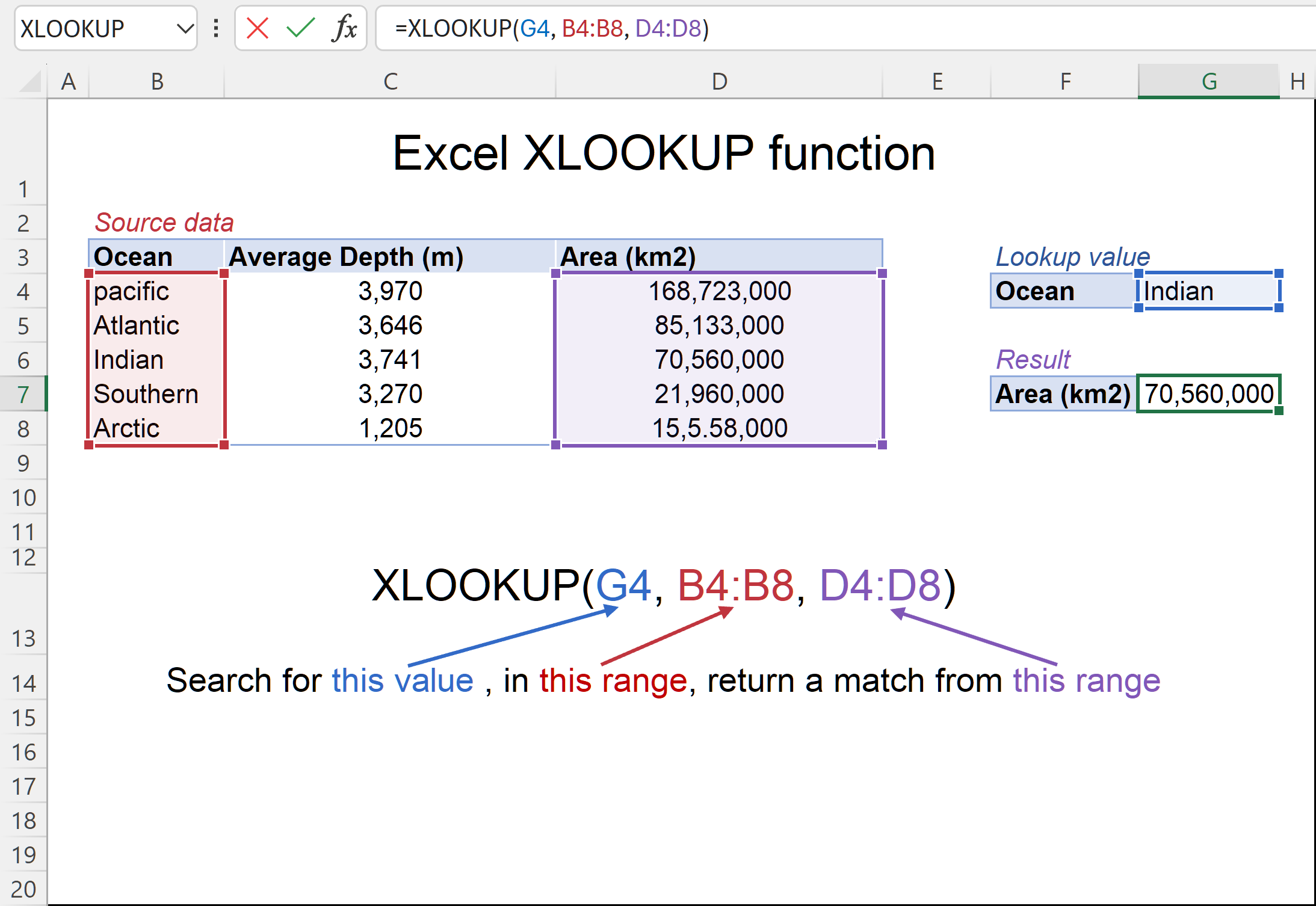
Supposing, you have a summary table with information about the five oceans on the Earth. You want to get the area of a specific ocean input in G4 (lookup_value). With the ocean names in B4:B8 (lookup_array) and areas in D4:D8 (return_array), the formula goes as follows:
=XLOOKUP(G4, B4:B8, D4:D8)
Translated into plain English, it says: search for the G4 value in B4:B8 and return a value from D4:D8 in the same row. No column index numbers, no sorting, no other ridiculous quirks of Vlookup! It just works :)
If needed, you can "hardcode" the lookup value directly in a formula like this:
=XLOOKUP("Indian", B4:B8, D4:D8)
How is XLOOKUP better than VLOOKUP?
XLOOKUP is a powerful function that surpasses VLOOKUP in many aspects. It offers more capabilities, versatility and efficiency. Here are the top 10 features that make it the ultimate lookup function in Excel:
- Vertical and horizontal lookup. The XLOOKUP function got its name due to its ability to look up both vertically and horizontally.
- Look in any direction: right, left, bottom or up. While VLOOKUP can only search in the leftmost column and HLOOKUP in the topmost row, XLOOKUP has no such limitations. The notorious left lookup in Excel is not a pain anymore!
- Exact match by default. In most situations, you will be looking for an exact match, and XLOOKUP returns it by default (unlike the VLOOKUP function that defaults to approximate match). Of course, you can get XLOOKUP to perform an approximate match too if needed.
- Partial match with wildcards. When you know only some part of the lookup value, not all of it, a wildcard match comes in handy.
- Search in reverse order. Earlier, to get the last occurrence, you had to reverse the order of your source data. Now, you simply set the search_mode argument to -1 to force your Xlookup formula to search from the back and return the last match.
- Return multiple values. By manipulating with the return_array argument, you can pull an entire row or column of data related to your lookup value.
- Search with multiple criteria. Excel XLOOKUP handles arrays natively, which makes it possible to perform lookup with multiple criteria.
- If error functionality. Traditionally, we use the IFNA function to trap #N/A errors. XLOOKUP incorporates this functionality in the if_not_found argument allowing to output your own text if no valid match is found.
- Column insertions/deletions. One of the most irritating issues with VLOOKUP is that adding or removing columns breaks a formula because the return column is identified by its index number. With XLOOKUP, you supply the return range, not number, meaning you can insert and remove as many columns as you need without breaking anything.
- Better performance. VLOOKUP could slow down your worksheets because it includes the entire table in calculations, which results in processing far more cells than actually needed. XLOOKUP handles only the lookup and return arrays that it truly depends on.
For more information, please see Difference between VLOOKUP and XLOOKUP.
How to use XLOOKUP in Excel - formula examples
The following examples demonstrate the most useful XLOOKUP features in action. Additionally, you will discover a couple non-trivial uses that will take your Excel lookup skills to a new level.
Look up vertically and horizontally
Microsoft Excel used to have two functions for different lookup types, each having its own syntax and usage rules: VLOOKUP to look vertically in a column and HLOOKUP to look horizontally in a row.
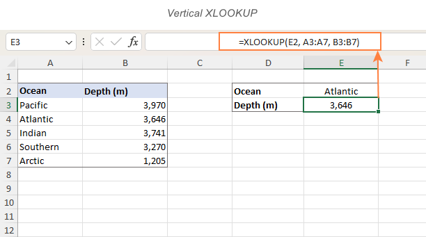
The XLOOKUP function can do both with the same syntax. The difference is in what you provide for the lookup and return arrays.
For v-lookup, supply columns:
=XLOOKUP(E2, A3:A7, B3:B7)
For h-lookup, enter rows instead of columns:
=XLOOKUP(I1, B1:F1, B2:F2)

Left lookup performed natively
In earlier versions of Excel, INDEX MATCH formula was the only reliable way to look to the left or above. Now, you no longer need to combine two functions where one would suffice. Just specify the target lookup array, and XLOOKUP will handle it without a problem regardless of its location.
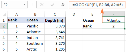
As an example, let's add the Rank column to the left of our sample table. The goal is to get the rank of the ocean input in F1. VLOOKUP would stumble here because it can only return a value from a column to the right of the lookup column. An Xlookup formula copes with ease:
=XLOOKUP(F1, B2:B6, A2:A6)
In a similar manner, you can look above when searching horizontally in rows.
XLOOKUP with exact and approximate match
The match behavior is controlled by the 5th argument called match_mode. By default, an exact match is performed.
Please pay attention that even when you choose an approximate match (match_mode set to 1 or -1), the function will still search for an exact match first. The difference is in what it returns if an exact lookup value is not found.
Match_mode argument:
- 0 or omitted - exact match; if not found - #N/A error.
- -1 - exact match; if not found - next smaller item.
- 1 - exact match; if not found - next larger item.
Exact match XLOOKUP
This is the option you probably use 99% of the time you do lookup in Excel. Since an exact match is XLOOKUP's default behavior, you can omit match_mode and supply only the first 3 required arguments.
In some situations, however, an exact match won't work. A typical scenario is when your lookup table does not contain all the values, but rather "milestones" or "bounds" like quantity-based discounts, sales-based commissions, etc.
Our sample lookup table shows the correlation between exam scores and grades. As you can see in the screenshot below, an exact match works only when the score of a particular student matches the value in the lookup table exactly (like Christian in row 3). In all other cases, an #N/A error is returned.
=XLOOKUP(F2, $B$2:$B$6, $C$2:$C$6)
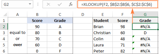
To get the grades instead of #N/A errors, we need to look for an approximate match as shown in the next example.
Approximate match XLOOKUP
To perform an approximate lookup, set the match_mode argument to either -1 or 1, depending on how your data is organized.
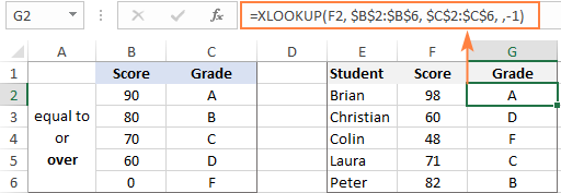
In our case, the lookup table lists the lower bounds of the grades. So, we set match_mode to -1 to search for the next smaller value when an exact match is not found:
=XLOOKUP(F11, $B$11:$B$15, $C$11:$C$15, ,-1)
For example, Brian has the score of 98 (F2). The formula searches for this lookup value in B2:B6 but cannot find it. Then, it searches for the next smaller item and finds 90, which corresponds to grade A:
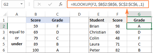
If our lookup table contained the upper bounds of the grades, we would set match_mode to 1 to search for the next larger item if an exact match fails:
=XLOOKUP(F2, $B$2:$B$6, $C$2:$C$6, ,1)
The formula searches for 98 and again cannot find it. This time, it tries to find the next larger value and gets 100, corresponding to grade A:
Tip. When copying an Xlookup formula to multiple cells, lock the lookup or return ranges with absolute cell references (like $B$2:$B$6) to prevent them from changing.
XLOOKUP with partial match (wildcards)
To perform a partial match lookup, set the match_mode argument to 2, which instructs the XLOOKUP function to process the wildcard characters:
- An asterisk (*) - represents any sequence of characters.
- A question mark (?) - represents any single character.
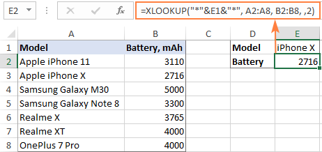
To see how it works, please consider the following example. In column A, you have a few smartphone models and, in column B, their battery capacity. You are curious about the battery of a certain smartphone. The problem is that you are not sure you can type the model name exactly as it appears in column A. To overcome this, enter the part that is definitely there and replace the remaining characters with wildcards.
For example, to get information about the battery of iPhone X, use this formula:
=XLOOKUP("*iphone X*", A2:A8, B2:B8, ,2)
Or, input the known part of the lookup value in some cell and concatenate the cell reference with the wildcard characters:
=XLOOKUP("*"&E1&"*", A2:A8, B2:B8, ,2)
Tip. If wildcards don't offer the precision you need, you can use XLOOKUP with regex match to search for more complex text structures, specific prefixes, or character sequences, etc.
XLOOKUP in reverse order to get last occurrence
In case your table contains several occurrences of the lookup value, you may sometimes need to return the last match. To have it done, configure your Xlookup formula to search in reverse order.
The direction of search is controlled be the 6th argument named search_mode:
- 1 or omitted (default) - searches from first to last value, i.e. top-to-bottom with vertical lookup or left-to-right with horizontal lookup.
- -1 - searches in reverse order from last to first value.
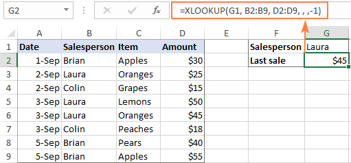
As an example, let's return the last sale made by a specific salesperson. For this, we put together the first three required arguments (G1 for lookup_value, B2:B9 for lookup_array, and D2:D9 for return_array) and put -1 in the 5th argument:
=XLOOKUP(G1, B2:B9, D2:D9, , ,-1)
Straightforward and easy, isn't it?
XLOOKUP to return multiple columns or rows
One more amazing feature of XLOOKUP is its ability to return more than one value relating to the same match. All is done with the standard syntax and without any extra manipulations!
From the below table, supposing you want to retrieve all the details pertaining to the salesperson in F2. What you need to do is supply a range containing several columns (B2:D7) for the return_array argument:
=XLOOKUP(F2, A2:A7, B2:D7)
You enter the formula in the top-left cell of the results range, and Excel automatically spills the results into adjacent blank cells. In our case, the returned array (G2:I2) consists of 1 row and 3 columns (Date, Item and Amount). Looking from another angle, we can say that XLOOKUP returns an entire row of data relating to the lookup value.

If you prefer to arrange the results vertically in a column, nest XLOOKUP into the TRANSPOSE function to flip the returned array:
=TRANSPOSE(XLOOKUP(G1, A2:A7, B2:D7))
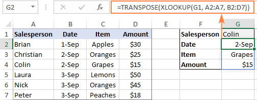
To return values from non-adjacent columns, nest the FILTER function in the return_array of XLOOKUP. A horizontal array {1,0,1} served to the include argument of FILTER determines which columns to filter out (0s) and which to return (1s).
=XLOOKUP(F2, A2:A7, FILTER(B2:D7, {1,0,1}))

It should be noted, however, that XLOOKUP cannot return multiple columns when the lookup_value argument is a range. In this case, you can use the combination of the CHOOSEROWS and XMATCH functions:
=CHOOSEROWS(B2:C10, XMATCH(E2:E4, A2:A10))

Similarly, you can return values from multiple rows when performing a horizontal lookup. To put it differently, you can return an entire column of data relating to your lookup value.
For example, to return all the values from the Amount column, use "Amount" (F1) as lookup_value, the range A1:D1 containing the column headers as lookup_array, and the range A2:D7 as return_array.
=XLOOKUP(F1, A1:D1, A2:D7)
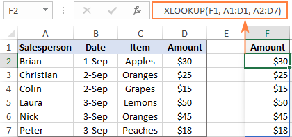
It’s important to ensure that you have enough blank cells to the right or down when using XLOOKUP to return multiple values, as a #SPILL! error will occur if there are not enough empty cells.
Tip. XLOOKUP can also be used to search for and replace values with other values that you specify. A example of such bulk replace can be found here: How to search and replace multiple values with XLOOKUP.
Note. If your lookup array contains multiple occurrences of the lookup value and you aim to return all matches, XLOOKUP cannot do that. In this case, you can use either:
- The FILTER function to return multiple matches in Excel 365 - 2021.
- A combination of INDEX, SMALL and ROW functions that works in any version: lookup multiple values in Excel.
XLOOKUP with multiple criteria
Another big advantage of XLOOKUP is that it handles arrays natively. Due to this ability, you can evaluate multiple criteria directly in the lookup_array argument:
How this formula works: The result of each criteria test is an array of TRUE and FALSE values. The multiplication of the arrays converts TRUE and FALSE into 1 and 0, respectively, and produces the final lookup array. As you know, multiplying by 0 always gives zero, so in the lookup array, only the items that meet all the criteria are represented by 1. And because our lookup value is "1", Excel takes the first "1" in lookup_array (first match) and returns the value from return_array in the same position.
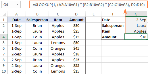
To see the formula in action, let's pull an amount from D2:D10 (return_array) with the following conditions:
- Criteria1 (date) = G1
- Criteria2 (salesperson) = G2
- Criteria3 (item) = G3
With dates in A2:A10 (criteria_range1), salesperson names in B2:B10 (criteria_range2) and items in C2:C10 (criteria_range3), the formula takes this shape:
=XLOOKUP(1, (B2:B10=G1) * (A2:A10=G2) * (C2:C10=G3), D2:D10)
Though the Excel XLOOKUP function processes arrays, it works as a regular formula and is completed with a usual Enter keystroke.
The XLOOKUP formula with multiple criteria is not limited to "equal to" conditions. You are free to use other logical operators as well. For example, to filter orders made on the date in G1 or earlier, put "<=G1" in the first criterion:
=XLOOKUP(1, (A2:A10<=G1) * (B2:B10=G2) * (C2:C10=G3), D2:D10)
For more examples, please see How to use XLOOKUP multiple criteria.
Double / nested XLOOKUP
To find a value at the intersection of a certain row and column, perform the so-called double lookup or matrix lookup. Yep, Excel XLOOKUP can do that too! You simply nest one function inside another:
How this formula works: The formula is based on XLOOKUP's ability to return an entire row or column. The inner function searches for its lookup value and returns a column or row of related data. That array goes to the outer function as the return_array.
For this example, we are going to find the sales made by a particular salesperson within a certain quarter. For this, we enter the lookup values in H1 (salesperson name) and H2 (quarter), and do a two-way Xlookup with the following formula:
=XLOOKUP(H1, A2:A6, XLOOKUP(H2, B1:E1, B2:E6))
Or the other way round:
=XLOOKUP(H2, B1:E1, XLOOKUP(H1, A2:A6, B2:E6))
Where A2:A6 are the salesperson names, B1:E1 are quarters (column headers), and B2:E6 are data values.

A two-way lookup can also be performed with an INDEX Match formula and in a few other ways. For more information, please see Two-way lookup in Excel.
If Error XLOOKUP
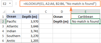
When the lookup value is not found, Excel XLOOKUP returns an #N/A error. Quite familiar and understandable to expert users, it might be rather confusing for novices. To replace the standard error notation with a user-friendly message, type your own text into the 4th argument named if_not_found.
Back to the very first example discussed in this tutorial. If someone inputs an invalid ocean name in E1, the following formula will explicitly tell them that "No match is found":
=XLOOKUP(E1, A2:A6, B2:B6, "No match is found")
Notes:
- The if_not_found argument traps only #N/A errors, not all errors.
- #N/A errors can also be handled with IFNA and VLOOKUP, but the syntax is a bit more complex and a formula is lengthier.
Case-sensitive XLOOKUP
By default, the XLOOKUP function treats lowercase and uppercase letters as the same characters. To make it case-sensitive, use the EXACT function for the lookup_array argument:
How this formula works: The EXACT function compares the lookup value against each value in lookup array and returns TRUE if they are exactly the same including the letter case, FALSE otherwise. This array of logical values goes to the lookup_array argument of XLOOKUP. As the result, XLOOKUP searches for the TRUE value in the above array and returns a match from the return array.
For example, to get the price from B2:B7 (return_array) for the item in E1 (lookup_value), the formula in E2 is:
=XLOOKUP(TRUE, EXACT(E1, A2:A7), B2:B7, "Not found")
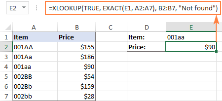
Note. If there are two or more exactly the same values in the lookup array (including the letter case), the first found match is returned.
Excel XLOOKUP not working
If your formula does not work right or results in error, most likely it's because of the following reasons:
XLOOKUP is not available in my Excel
The XLOOKUP function is not backward compatible. It's only available in Excel for Microsoft 365 and Excel 2021, and won't appear in earlier versions.
XLOOKUP returns wrong result
If your obviously correct Xlookup formula returns a wrong value, chances are that the lookup or return range "shifted" when the formula was copied down or across. To prevent this from happening, be sure to always lock both ranges with absolute cell references (like $A$2:$A$10).
XLOOKUP returns #N/A error
An #N/A error just means the lookup value is not found. To fix this, try searching for approximate match or inform your users that no match is found.
XLOOKUP returns #VALUE error
A #VALUE! error occurs if the lookup and return arrays have incompatible dimensions. For instance, it is not possible to search in a horizontal array and return values from a vertical array.
XLOOKUP returns #REF error
A #REF! error is thrown when looking up between two different workbooks, one of which is closed. To fix the error, simply open both files.
As you have just seen, XLOOKUP has many awesome features that make it THE function for almost any lookup in Excel. I thank you for reading and hope to see you on our blog next week!
Practice workbook for download
Excel XLOOKUP formula examples (.xlsx file)
 by
by
103 comments
I have this XLookup formula that is pulling data from a table I created for a yearly financial tracking program. It works perfectly. I have the table on every sheet which works but isn't very pretty.
I would like to have one sheet in my workbook just for the table. Almost every sheet would need access to that sheet- let's call it Ref.
How would I rewrite this formula to include that separate page?
=XLOOKUP(H15, $Q$3:$Q$3467, $R$3:$R$3467, uncategorized)
My dataset:
-Dates vertically aligned (i.e., going down the column)
-Locations going horizontally (i.e. row header)
-Names are populated in the table (it is a very large dataset with thousands of locations and names)
Example:
Date McDonalds Burger King Movie Theatre
2/13/2024 Kathy Cindy John
2/14/2024 Pops Matt Karen
2/15/2024 Jesus Guy Girl
2/16/2024 Matt Dude Girl
I want to return the location when the name and date match.
Example of desired return:
Input: Matt
2/13/2024 Not Found
2/14/2024 Burger King
2/15/2024 Not Found
2/16/2024 McDonalds
Thank you so much for your help.
Hi! If I understand your task correctly, this article may be helpful: INDEX MATCH MATCH in Excel for two-dimensional lookup.
If E1="Matt", the formula in E2 might look like this:
=IFERROR(INDEX($B$1:$E$1,, MATCH($H$1, INDEX($B$2:$E$5, MATCH(A2,$A$2:$A$5,0),),0)),"")
You can copy this formula down along the column E.
Great tutorial - thanks.
Question: I have up to 24 rows of scores in a 5 week tournament. Sometimes, players will notify me that they can't play.
My premise is this: Given a player-substitution list of a column of names and a row of 5 dates. The absent day would have an "X".
I want to use xlookup and conditional formatting to color the score-sheet player/date intersection if blank or no-color if a score is in it.
Score sheet: names:B15:B60, date: D5:H5, scores: D15:H60.
Substitute table can be either of 2 ways:
(1)a column of names with a row of dates and 'X' where the substitution is needed (preferred)
OR
(2)Column of names with absent date in one of 5 columns.
My conditional statement is (D15): =NOT(AND(ISBLANK(D15),(XLOOKUP($B15,$R$41:$R$43,XLOOKUP($D$5,$S$41:$V$41,$S$41:$V$43))))) using method 2.
Using conditional formatting I'm not able to propagate easily in 24 rows x 5 dates(dates)
Hello Chuck!
If you want to highlight empty cells in a range of Excel values with a color, you can try to use following guidelines: Excel conditional formatting for blank cells.
I hope it’ll be helpful. If this is not what you wanted, please describe the problem in more detail.
Hello Alexander
Thank you for your tutotial however I have a problem dealing with data returned from a loaded Power Query worksheet.
The original source data is from a VB created CSV file.
The data from the CSV is taken into Power Query and without doing anything to it, it is loaded to an excel file. the loading process auto creates the worksheet and names the tab.
All the loaded data comes into the excel file formatted as "General" even though there is both numbers, text and dates in the source data.
In another tab of the excel file I extract the required information from the loaded worksheet using Xlookup. I use the following formula =XLOOKUP(TEXT($K530,"00"),'RTB'!$A:$A,'RTB'!C:C) I get the correct data using this formula and I use multiple permutations of this formula. Thereare 1000 rows and 50 columns in the source data and this will auto expand when necessary
The data provided by XLookup is pulled into multiple long lists and each list needs to be totaled. However I cannot use the sum function to do this as it always returns 0 which is totally incorrect. However the +(plus) does work but that's untenable to use with 50 or more rows in any one list and there are many lists required.
Is there any solution to this sum problem of getting the sum function to work?
I have tried may format options to the data provided by Power Query, but to no avail.
The data source changes continually and the lookup formula output is dynamic to that source
I would be most grateful if you could please help.
Rgds
Michael
Hello Michael!
I assume the numbers you want to sum are written as text. So SUM will return zero. But any mathematical operation will convert this text to numbers. So you can sum them manually. Please use the following guide: How to convert text to number in Excel.
Why is my formula not working? #VALUE! returned. =XLOOKUP(1,('Q3'!A2:AG100=A22)*('Q3'!G2:AF2=M2),'Q3'!N2:N100)
Hello Mona!
You cannot multiply arrays of this size. You cannot multiply an array of 33 columns by an array of 26 columns. Read more about working with arrays. Click here: Excel array formulas, functions and constants - examples and guidelines.
Hello...... I'm not using the * to multiple, I am using as: "AND operator is the asterisk (*) which is the multiplication symbol. It instructs Excel to return TRUE if ALL of the conditions evaluate to TRUE."
Hi! For a better understanding, I recommend that you read this section carefully: AND and OR operators in array formulas. You can also find useful information in this article: Excel XLOOKUP with multiple criteria.
why does my vlookup cell return not an error or the correct value but simply the text of the formula? So the cell would return: =vlookup(A2,b2,d20,3,false)
Hi! The formula is written incorrectly. You can find the examples and detailed instructions here: Excel VLOOKUP function tutorial with formula examples.
Typo: should be cell formula: =vlookup(A2,b2:d20,3,false)
Hi Svetlana and Ablebits Team,
I trying to use your tutorial to understand how to return a value for a specific month and account number.
Account January February March April
A 100 200 300 400
B 500 600 700 800
C 900 1,000 1,100 1,200
D 1,300 1,400 1,500 1,600
E 1,700 1,800 1,900 2,000
For example, the value for Account 'D' in March is 1,500. I would like to populate a separate table such as below.
Account January February March April
A
B
C
D
E
Thanks and much appreciated,
Daniel
Hi! Your two tables have the same format. Fill the second table using the usual cell references from the first table. To search by row and column, use the following instructions: INDEX MATCH MATCH in Excel for two-dimensional lookup. Hope this is what you need.
Can XLOOKUP be used to find and replace values in the middle of a string? I have about 12 cells that say "01-xx-234000." In a separate cell on each of those lines, there's a corresponding 4 character code. All of those 4 character codes and the numbers that correspond to the "xx" in the string are referenced in a pivot table. I'd like to use XLOOKUP to replace the "xx" so that the long strings can have the correct 2 digit numbers. (The xx would be replaced and the strings would read 01-12-234000, 01-13-234000, etc etc.) Is that possible?
Hi! To change the text string in a cell, you need the SUBSTITUTE or REPLACE functions. The XLOOKUP function can only search for data. Look for the example formulas here: Using REPLACE and SUBSTITUTE functions in Excel.
There is not enough information to give you a formula.
Can we do XLOOKUP with a value instead of cell reference?
for example
=XLOOKUP("Saturday", A2:A20, D2:D20)
Hi! Yes, you can use a value instead of a cell reference for the search criteria.
Hi, I'm trying to pull multiple numbers from an excel page to add together into one cell. It seems like xlookup won't work for that, correct?
I have a page with types of expenses (P for payroll, D for disbursements, O for operations, etc.) and I would like to pull all amounts that correspond to that letter added into one cell. A separate page has amounts paid for each vendor, and I need to organize them into one amount in one cell.
First page
P (total)
D (total)
O (total)
Second page
P 300.00
O 2000.00
P 500.00
D 1400.00
O 8000.00
D 2400.00
Hi! To find the sum of values that match certain criteria, use the SUMIF function.
For example:
=SUMIF(A1:A20,"P",B1:B20)
If the values are on another worksheet, use external references as described in this guide: Excel reference to another sheet or workbook (external reference).
Hello,
Excellent information provided, however I can't seem to build the formula to work for what I need.
I have a table with three different headers determining information, laid out as below:
| SUPPORT | SUPPORT | SECURITY | SECURITY
-------------------------------------------------------------------
| Full | Co-op | Full | Co-op
-------------------------------------------------------------------
JAN | 10 | 20 | 30 | 40
FEB | 15 | 45 | 50 | 45
I am trying to use XLOOKUP to pull the numbers by matching the data in the first Column, and the first two Rows, i.e: I want to be able to pull the number for 'Full' 'SUPPORT' 'JAN', and pull a different number for 'Co-op' 'SUPPORT' 'JAN'
I don't think this is actually possible the way I'm trying at least, but would appreciate anyone's advice on how to make it work.
Hello! The XLOOKUP function cannot help you in your task. It cannot select several columns by the first condition and then select among them the required column by the second condition. Use FILTER function to select a column in the table that matches both conditions. Then use INDEX MATCH to find the third condition in column A and extract the corresponding value.
=INDEX(FILTER(B1:E4,(B2:E2=H2)*(B1:E1=H1)),MATCH(H3,A1:A4,0),1)
H1= SUPPORT
H2= Co-op
H3= FEB
Hope this is what you need.
Hello, really like your article.
As a newbie to the XLOOKUP function I understand the basics, where I am struggling is when I have a set of two criteria (Data & Employee number) that need to search against two different spreadsheet tabs. One tab contains a list of company employees and the other tab a list of contractors. I would like the formula to basically look at the two criteria and search the company employees tab, and if not found search the contractor tab.....how might that formula look?
Any help would be greatly appreciated!
Thanks
Hi! I recommend reading this guide: VLOOKUP with IF statement in Excel and VLOOKUP across multiple sheets in Excel with examples. You can do the same with the XLOOKUP function.
Realized I did not explain what I am looking for....I am trying to identify the name of the person who matches the two criteria (Date & Employee number). Each tab (company employees and contractors) has a date and number applied to there names. I am trying to pull that information, on another tab, into a single list of names containing both company employees and contractors using the XLOOKUP function.
If you want to extract multiple values from each sheet based on two criteria, I suggest using these guidelines: How to Vlookup multiple values in Excel with criteria. To get a list of names, we can also use the FILTER function as described in this article: Excel FILTER function - dynamic filtering with formulas.
Hello,
I am asking XLOOKUP to do a lookup only I get the #NAME?. I honestly can't see what is wrong with my formula.
=XLOOKUP(K:K,'GPS-Data'!A:A,'GPS-Data'!B:B)
Hi! This #NAME? error means that there is no such function in your Excel. See the function description at the beginning of this article.
Hello. This is so useful, thank you.
Is there a way of getting the XLOOKUP to look at and return a value from a different range if the range it is looking at is empty? For example, I am asking it to return a value from B4:T4, by looking up K61 in B12:T12. If B12:T12 is empty, i'd like it to look and to return a value from B9:T9 instead. Is this possible?
My main formula is =XLOOKUP(K61,B12:T12,B4:T4,"") and to solve my problem I have tried =IF(XLOOKUP(K61,B12:T12,B4:T4)="",XLOOKUP(K61,:B9:T9,B4:T4)) but it keeps returning NA when there is definitely a value in B9:T9. Any help greatly appreciated. Thanks
Hello! The following tutorial should help: IF VLOOKUP in Excel: Vlookup formula with If condition. You can do the same with the XLOOKUP function. For example,
=IF(ISNA(XLOOKUP(K61,B12:T12,B4:T4)), XLOOKUP(K61,B9:T9,B4:T4), XLOOKUP(K61,B12:T12,B4:T4))
I hope it’ll be helpful.
Hi,
=XLOOKUP("*B1*",Ordering!L:L,Ordering!A:A, "", 2)
How would I adjust that formula so that the search key(from a drop down menu in B1) returns partial matches eg. JER / TK. from the search range?
Hi! To find a partial match in text values, use these guidelines: How to find substring in Excel. For example:
=XLOOKUP(TRUE,ISNUMBER(SEARCH("B1",Ordering!L:L,Ordering!A:A)), "", 2)
Hi! I am trying to create a formula using XLOOKUP that can generate a column average and also work with different quantities of columns (this formula will address survey responses, so, one worksheet may have 10 columns that need to be "looked up", and one may have three). Is there a formula that you would recommend?
Thanks,
Caroline
Hi! The XLOOKUP formula cannot generate any value. It can only find an existing value based on the criteria. To calculate the average value, use these guidelines: How to calculate average in Excel: formula examples, Excel AVERAGEIF function to average cells with condition
Thank you for this very informative article. I am trying to use xlookup to return the smallest of values in the return range where the lookup value occurs multiple times in the lookup range. It looks like it just returns the first one it finds. Is there a way to use the xlookup function as is, or to nest another formula to control which value is returned?
Example:
=XLOOKUP("A-B-C-D",A:A,B:B)
Tag | Sequence
A-B-C-D | 5
C-D-T-G | 4
G-H-E-H | 2
A-B-C-D | 3
B-T-R-D | 1
"A-B-C-D" occurs twice, but would like to return the smaller of the two value (3), instead of (5) as it currently does, without having to change the sort of the table.
Thank you,
-Andres
Hi!
To search by multiple criteria, use the INDEX MATCH functions. You can learn more about MINIFS function in Excel in this article on our blog.
Try this formula:
=INDEX(B1:B5,MATCH(1,(A1:A5="A-B-C-D") * (B1:B5=MINIFS(B1:B5,A1:A5,"A-B-C-D")),0))
Hello,
I was particularly interested in the above section on "XLOOKUP to return multiple columns or rows".
Can you tell me, is the return array limited to adjacent columns (as your example per B2:D7 returns information from columns B, C and D.)?
Or is it possible to return information from a table which has many columns but you only want info from for example B, F, K?
Thanks, Janek
Hello! Extract values from all adjacent columns, for example B:D. To get values from only a few columns, for example from B and D, use the CHOOSECOLS function.
Here is an example of this formula:
=CHOOSECOLS(XLOOKUP(F3, A3:A8, B3:D8),1,3)
For more information, please visit: CHOOSECOLS function in Excel to get columns from array or range.
Thank you, that is almost perfect for what I need, though I think I see that when CHOOSECOLS is used, the XLOOKUP lookup value must be a single cell address and not an array itself.
I am trying to work out this formula =IF(A2>0, "Non Compliance","Compliance") but I want to exclude blank cells. How can I do that?
To add a second condition, use IF OR statement.
If I understand your task correctly, try the following formula:
=IF(OR(A2>0, ISBLANK(A2)), "Non Compliance","Compliance")
For more information, please visit: ISBLANK function in Excel to check if cell is blank
Can a nested Xlookup return a result based on criteria in two different columns? I noticed that the most successful results are when there is one horizontal and one vertical.
Hi Paul,
Sure, it can. Please check the "XLOOKUP with multiple conditions" example in this tutorial.
Hello!
You can read how to do a 2D search by rows and columns in this article - Excel INDEX MATCH MATCH and other formulas for two-way lookup