If you've been following this blog for a while, you may remember QUERY function for Google Sheets. I mentioned it as a possible solution for a couple of cases. But those are far from enough to uncover its full potential. Today, it's high time we get to know this spreadsheets superhero properly. And guess what – one equally noteworthy tool will also be there :)
Did you know that Google Sheets QUERY function is considered to be the most powerful one in spreadsheets? Its peculiar syntax favours tens of different operations. Let's try and break its parts down to learn them once and for all, shall we?
Syntax of Google Sheets QUERY function
At first glance, Google Sheets QUERY is just another function with 1 optional and 2 required arguments:
- data is the range to process. Required. Everything is crystal clear here.
Note. Only one small reminder here established by Google: each column should contain one type of data: textual, or numeric, or boolean. If there are different types, QUERY will work with the one that occurs the most. Other types will be considered as empty cells. Strange, but keep that in mind.
- query is the way to process the data. Required. This is where all the fun begins. Google Sheets QUERY function uses a special language for this argument: Google Visualization API Query Language. It's written in a way similar to SQL. Basically, it's a set of special clauses (commands) used to tell the function what to do: select, group by, limit, etc.
Note. The entire argument must be enclosed in double-quotes. Values, in their turn, should be wrapped in quotation marks.
- headers is optional for when you need to indicate the number of header rows in your data. Omit the argument (as I do below), and Google Sheets QUERY will assume it based on the contents of your table.
Now let's dig deeper into the clauses and whatever they do.
Clauses used in Google Sheets QUERY formulas
Query language consists of 10 clauses. They may frighten at first glance, especially if you're not familiar with SQL. But I promise, once you get to know them, you will get a powerful spreadsheet weapon at your disposal.
I'm going to cover each clause and provide formula examples using this list of imaginary students and their paper subjects:
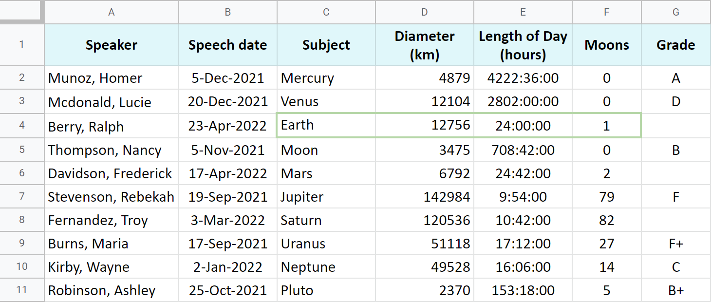
Yep, I'm one of those weirdos who think Pluto should be a planet :)
Tip. Several clauses can be used within one Google Sheets QUERY function. If you nest them all, make sure to follow the order of their appearance in this article.
Select (all or specific columns)
The very first clause – select – is used to tell what columns you need to return with Google Sheets QUERY from another sheet or table.
Example 1. Select all columns
To fetch each and every column, use select with an asterisk – select *
=QUERY(Papers!A1:G11,"select *")
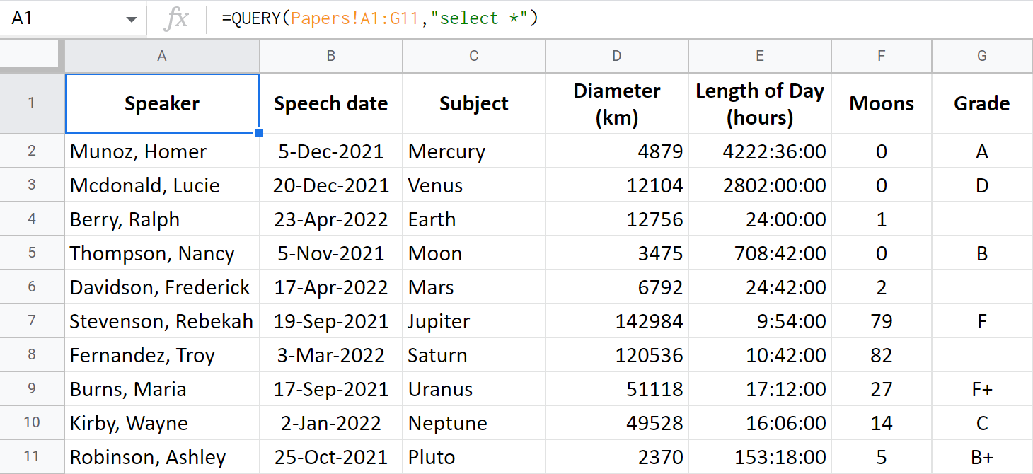
Tip. If you omit the select parameter, Google Sheets QUERY will return all columns by default:
=QUERY(Papers!A1:G11)
Example 2. Select specific columns
To pull only certain columns, list them after the select clause:
=QUERY(Papers!A1:G11, "select A,B,C")
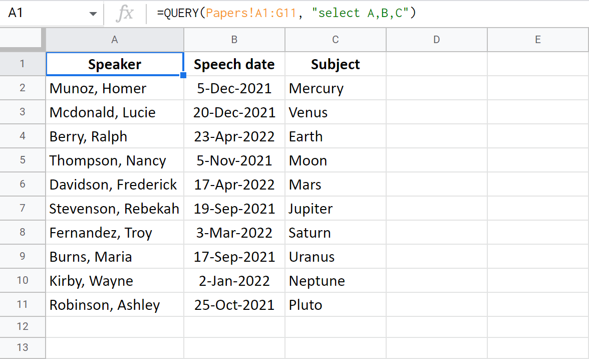
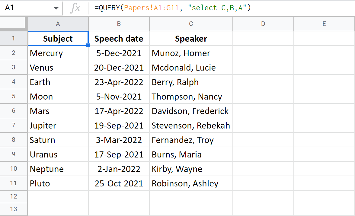
Tip. The columns of interest will be copied in the same order you mention them in the formula:
=QUERY(Papers!A1:G11, "select C,B,A")
Google Sheets QUERY – Where clause
Google Sheets QUERY where is used to set the conditions towards the data you want to get. In other words, it acts as a filter.
If you use this clause, QUERY function for Google Sheets will search columns for values that meet your conditions and fetch all matches back to you.
Tip. Where can function without the select clause.
As usual, to specify conditions, there are sets of special operators for you:
- simple comparison operators (for numeric values): =, <>, >, >=, <, <=
- complex comparison operators (for strings): contains, starts with, ends with, matches, != (doesn't match / doesn't equal to), like.
- logical operators to combine several conditions: and, or, not.
- operators for blank / not empty: is null, is not null.
Tip. If you're upset or worried about having to deal with such a huge number of operators again, we feel you. Our Filter and Extract Data will find all matches and build QUERY formulas in Google Sheets for you if necessary.
Let's see how these operators behave in formulas.
Example 1. Where with numbers
I will add where to my Google Sheets QUERY from above to get the info on those planets that have more than 10 moons:
=QUERY(Papers!A1:G11,"select A,B,C,F where F>=10")

Tip. I also mentioned column F to fetch just to make sure the criterion is met. But it's completely optional. You don't have to include columns with conditions into the result:
=QUERY(Papers!A1:G11,"select A,B,C where F>=10")
Example 2. Where with text strings
- I want to see all rows where the grade is either F or F+. I will use the contains operator for that:
=QUERY(Papers!A1:G11,"select A,B,C,G where G contains 'F'")
Note. Don't forget to surround your text with quotation marks.
- To get all rows with F only, just replace contains with an equal sign (=):
=QUERY(Papers!A1:G11,"select A,B,C,G where G='F'") - To check the papers that are yet to be delivered (where the grade is missing), check column G for blanks:
=QUERY(Papers!A1:G11,"select A,B,C,G where G is null'")
Example 3. Where with dates
Guess what: Google Sheets QUERY has even managed to tame dates!
Since spreadsheets store dates as serial numbers, usually, you have to resort to the help of special functions like DATE or DATEVALUE, YEAR, MONTH, TIME, etc.
But QUERY has found its way around dates. To enter them properly, simply type the word date and then add the date itself formatted as yyyy-mm-dd: date '2022-01-01'
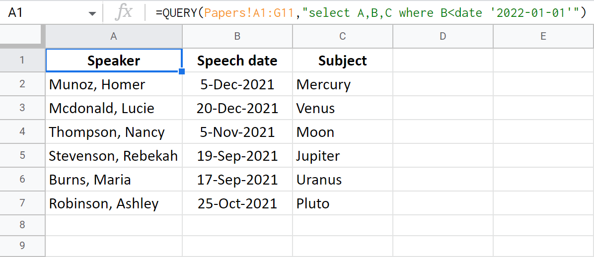
Here's my formula to get all rows with a Speech date before 1 Jan 2022:
=QUERY(Papers!A1:G11,"select A,B,C where B<date '2022-01-01'")
Example 4. Combine several conditions
To use a certain period of time as a criterion, you will need to combine two conditions.
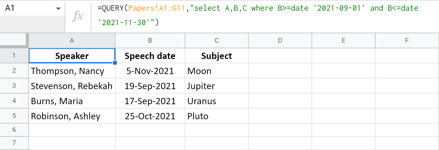
Let's try and retrieve those papers that were delivered in Autumn, 2019. The first criteria should be a date on or after 1 September 2021, the second — on or before 30 November 2021:
=QUERY(Papers!A1:G11,"select A,B,C where B>=date '2021-09-01' and B<=date '2021-11-30'")
Or, I can select papers based on these parameters:
- before 31 December 2021 (B<date '2021-12-31')
- have either A or A+ as a grade (G contains 'A')
- or B/B+ (G contains 'B')
=QUERY(Papers!A1:G11,"select A,B,C,G where B<date '2021-12-31' and G contains 'A' or G contains 'B'")

Tip. If your head is about to explode already, don't give up just yet. There's a tool that is perfectly capable of building all these formulas for you, no matter the number of criteria. Jump right to the end of the article to get to know it.
Google Sheets QUERY – Group By
Google Sheets QUERY group by command is used to concatenate rows. However, you should use some aggregate functions in order to summarize them.
Note. Group by must always follow the select clause.
Unfortunately, there's nothing to group in my table as there are no recurring values. So let me adjust it a bit.
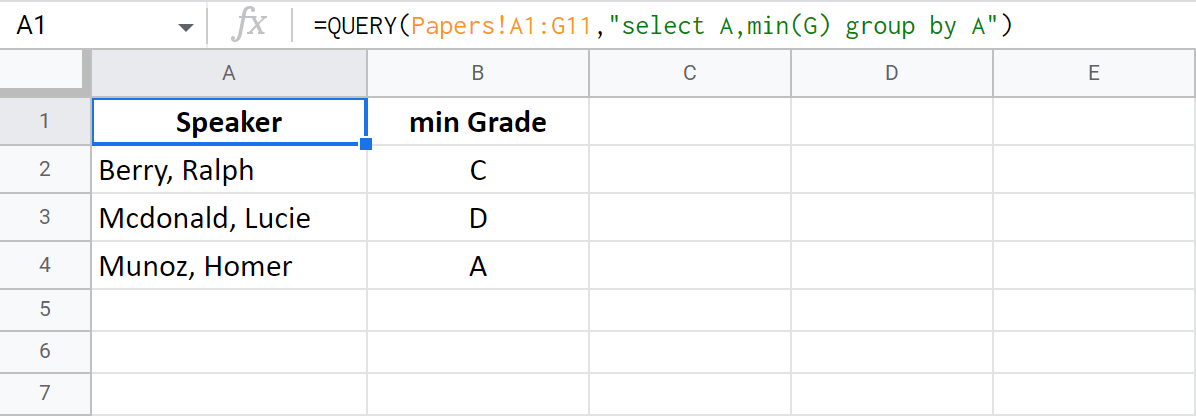
Suppose, all the papers are to be prepared by 3 students only. I can find the highest grade each student got. But since they are letters, it is the MIN function I should apply to column G:
=QUERY(Papers!A1:G11,"select A,min(G) group by A")
Note. If you don't use an aggregate function with any column in the select clause (column A in my example), you must duplicate them all in the group by clause.
Google Sheets QUERY – Pivot
Google Sheets QUERY pivot clause works the other way around, if I may say so. It transposes data from one column to a row with new columns, grouping other values accordingly.
For those of you dealing with dates, it can be a real discovery. You'll be able to get a quick glance at all the distinct years from that source column.
Note. When it comes to pivot, every column used in the select clause should be covered with an aggregate function. Else, it should be mentioned in the group by command following your pivot.
Remember, my table now mentions only 3 students. I'm going to make the function tell me how many reports each student made:
=QUERY(Papers!A1:G11,"select count(G) pivot A")

Google Sheets QUERY – Order By
This one is pretty easy :) It is used to sort the outcome by the values in certain columns.
Tip. All previous clauses are optional when using order by. I use select to return fewer columns for demonstration purposes.
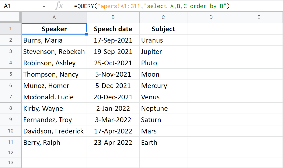
Let's go back to my original table and sort reports by speech date.
This next Google Sheets QUERY formula will get me columns A, B and C, but at the same time will sort them by date in column B:
=QUERY(Papers!A1:G11,"select A,B,C order by B")
Tip. You can learn everything about sorting data (by date, colors, etc.) in Google Sheets in this article.
Limit
What if I told you, you don't have to bring each and every row into the result? What if I told you that Google Sheets QUERY can pull only a certain amount of the first matches it finds?
Well, the limit clause is designed to help you with that. It limits the number of rows to return by the given number.
Tip. Feel free to use limit without other previous clauses.
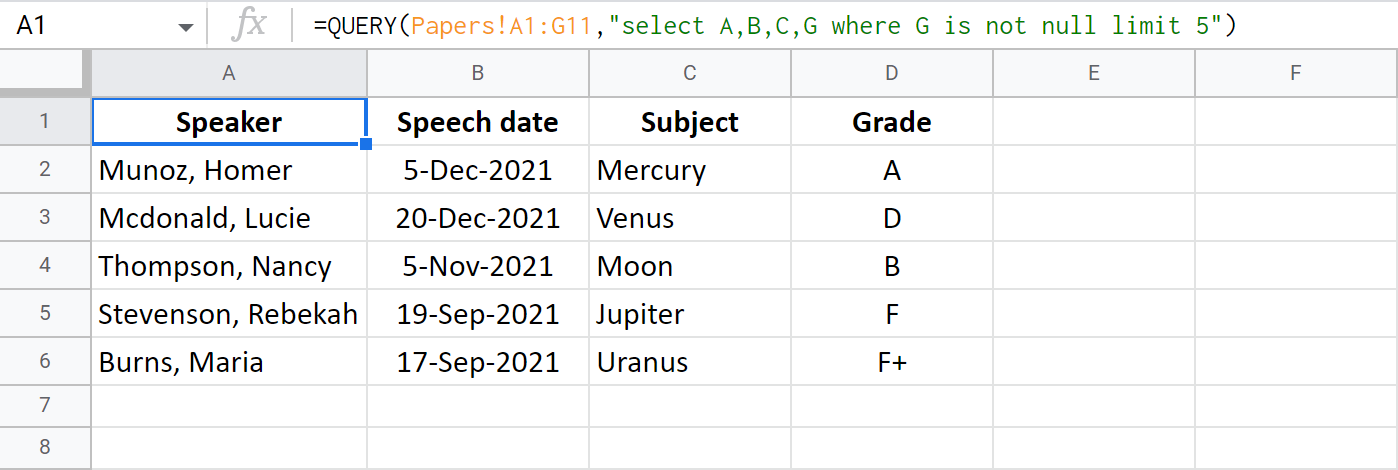
This formula will show the first 5 rows where the column with grades contains a mark (is not empty):
=QUERY(Papers!A1:G11,"select A,B,C,G where G is not null limit 5")
Offset
This clause is kind of opposite to the previous one. While limit gets you the number of rows you specify, offset skips them, retrieving the rest.
Tip. Offset also doesn't require any other clauses.
=QUERY(Papers!A1:G11,"select A,B,C,G where G is not null offset 5")

If you try and use both limit and offset, the following will happen:
- Offset will skip rows at the beginning.
- Limit will return a number of the following rows.
=QUERY(Papers!A1:G11,"select A,B,C,G where G is not null limit 3 offset 3")
Out of 11 rows of data (the first one is a header and QUERY function in Google Sheets does a nice job understanding that), offset skips the first 3 rows. Limit returns 3 next rows (starting from the 4th one):

Google Sheets QUERY – Label
Google Sheets QUERY label command lets you change header names of the columns.
Tip. Other clauses are optional for label as well.
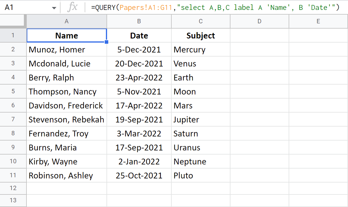
Put the label first, followed by the column ID and a new name. If you rename few columns, separate each new pair of column-label by a comma:
=QUERY(Papers!A1:G11,"select A,B,C label A 'Name', B 'Date'")
Format
The format clause makes it possible to alter the format of all values in a column. For that, you will need a pattern standing behind the desired format.
Tip. The format clause can also play solo in the Google Sheets QUERY.
=QUERY(Papers!A1:G11,"select A,B,C limit 3 format B 'mm-dd, yyyy, ddd'")

Tip. I mentioned some date formats for Google Sheets QUERY in this blog post. Other formats can be taken directly from spreadsheets: Format > Number > More Formats > Custom number format.
Options
This one is used to set some additional settings for the outcome data.
For example, such command as no_values will return formatted cells only.
The quickest way to build QUERY formulas – Filter and Extract Data
However powerful the QUERY function in Google Sheets is, it may require a learning curve to get ahold of. It's one thing to illustrate each clause separately on a small table, and completely another to try and build everything correctly with a few clauses and a much bigger table.
That's why we decided to dress Google Sheets QUERY up in a user-friendly interface and make it the add-on: Filter & Extract Data.
Why Filter & Extract Data is better than formulas?
Well, with the add-on there's absolutely no need to:
- figure out anything about those clauses. It's really easy to create lots of complex conditions in the add-on: as many as you need despite their order to fetch as many matches as you need.
Note. At the moment, the following clauses were incorporated into the tool: select, where, limit, and offset. If your task requires other clauses as well, please comment below – perhaps, you'll help us improve ;)
- know how to enter operators: just pick the one from a drop-down list.
- puzzle over the correct way to enter date and time. The add-on lets you enter them as you used to based on your spreadsheet locale.
Tip. There's always a hint available in the tool with examples of different data types.
As a bonus, you'll be able to:
- preview both the result and the formula
- make quick adjustments to your criteria
- select a place for the result
- insert the result as both QUERY formula or as values
I'm not kidding, see for yourself:
I hope you will give Filter & Extract Data a chance and install it to your Google Sheets.
This tutorial will also help you get started.
And don't hesitate to share your feedback, especially if there's something about it you don't like!
 by
by
162 comments
Hi guys, thanks so much for this walk through, I learned a lot! I am wondering if there is a way to format the query results in a table right away. So for instance, one of the source data columns is a dropdown with multiple selects. When the data is displayed in the query results, the multiple selections are displayed as comma separated text. Is it possible to convert query data directly into a table, to retain the functionality and sorting/filtering?
Scenario: i have a stocklist with a range of suppliers. Some items I can get from multiple suppliers. So I created the query to populate a reordering list once items in the inventory fall below a threshold value. The query function is great, because i can select the columns for the item name, its code, quantity to order, the price and the suppliers - all the info I need when doing my reordering. However, if the results were in a table, then I would also be able to filter by suppliers.
For example: Items 1 and 2 can be purchased at Samsons, Items 3 and 4 can be ordered from Harveys and Item 5 can be ordered from both. In a table, I would sort or filter by supplier to get the list for each place. As it is at the moment, even if I apply sort and filter on the column headers, Item 5 doesn't 'work' because it shows in the results as "Harveys, Samsons" rather than the category (or tag) that is such a great function of the Google Sheets table multiple select dropdown.
This is surprisingly hard to explain but I hope it makes some sort of sense. If it is possible to autoformat Query results into a table that would be great to know, thank you!
Formulas in Google Sheets can not return a real Table object and preserve multi-select dropdown like “chips.” QUERY and all other function can returns plain values only, therefore the pill-shaped chips are flattened to the text “Harveys, Samsons,” and the automatic filter/sort that tables give you can’t be generated by a formula. You have to create the table after the data is in place, or work from the original data instead of a formula spill range. While those "cool features" like chips, dropdown and so on look great and visually make the table clearer, I use them only for dashboard because those features limit your data processing.
I am trying to pull the data from a column in another sheet if a range of columns contains the information in my reference cell and equals a number in another column. This is the formula I am using. What am I doing wrong?
=query(Sheet5!A:O, "select A where J1:O100 contains'"&$A2&"' and F=1",0)
Hi
It's a good question! You're really close, but there are a couple of important points to correct:
1. In QUERY(), you can’t use a range like J1:O100 in the where clause, QUERY expects a single column for each condition.
2. Also, CONTAINS only works for a single column, not across multiple columns at once.
To solve your problem, you need to use the 'and' and 'or' operators.
=QUERY(Sheet5!A:O, "select A where (J contains '"&$A2&"' or O contains '"&$A2&"') and F = 1", 0)
I highly recommend using our Filter & Extract add-on. It was especially designed to help with syntax and complex logic.
Hello,
I have a column containing due date in one tabsheet and a cell containing the date of the day in the active one.
I would like to query all tasks related to : ("todays date" minus "due date") < 7 days
I tried : =QUERY(Planning!$A:$S;"select E where '"NB.JOURS.OUVRES(date "I;'"M1)<7")
Any idea would be greatly appreciated !
Thanks,
Hello Cédric,
For me to be able to help you, please share an editable copy of your sheet and your formula with us (support@apps4gs.com). Also, please include the second sheet with the result you expect to get. The result sheet is of great importance as it gives us a better understanding than any text description. I kindly ask you to shorten the tables to 10-20 rows.
Note. We keep that Google account for file sharing only and don't monitor its Inbox. Do not email there. Once you share the file, just confirm by replying to this comment.
I'll look into your task and try to help.
Hi,
When I do a query with the following formula =query(Data!A2:F235,"Select D where A contains 'A8'")
it lists everything in one cell. If I take out the where portion it lists all of column D in a column, but when I add the where statement it just puts all matches into one cell with spaces in between.
A8 is a dropdown that I'm referencing. If I put ,0 before the ) it give #N/A, if I put a number there, it will give the number of matches equal to the number I put in, but they're still in one cell.
What I want to do is list all matches from column A and then list all of the data from the same row from Column D. Bonus points if only lists the unique values to save me a step (dropdowns seem to do this by default, so if I can reference the cell that the formula is in that would work).
Ultimately, I'm making multiple dependent dropdowns (3 for now, but possibly 5, lets name them A, B, C, D, and E) and I have multiple choices in dropdown B are in multiple choices from dropdown A. So when I get to dropdown C I need to reference things in both dropdown A and B.
I had figured it all out on excel using filters, but iPads don't do data validation or VBA macros, so now I have to try and figure it out for sheets.
Hi DJ,
For me to be able to help you, please share an editable copy of your sheet and your formula with us (support@apps4gs.com).
Also, please include the second sheet with the result you expect to get. The result sheet is of great importance as it gives us a better understanding than any text description.
Please don't worry if you have confidential information there, we never disclose the data we get from our customers and delete it as soon as the problem is resolved. Or you can replace any important information with some irrelevant data, just keep the format.
Note. We keep that Google account for file sharing only and don't monitor its Inbox. Do not email there. Once you share the file, just confirm by replying to this comment.
I'll look into your task and try to help.
Hi,
Is there a way to SELECT a range of columns and have the WHERE clause refer to a Column outside that range? EX: query({'New'!A:BD},"Select Col1 through Co26 WHERE (Col55='No' or Col55='#N/A') AND Col56=True") . Columns 27 through 56 should not be part of the dataset returned.
Hi MBurke,
You can easily tell the Select clause which columns to return, but you must indicate the whole range as the first argument – data – to be able to reference other columns for conditions. Please look through the Select & Where sections for examples.
Hi Nathalia!
I'm using QUERY in combination with IMPORTRANGE. Unfortunately I can either use select *, or, if I select columns with Col1, Col2, it is limited to 3 cols max, so when I try to use "select Col1, Col2, Col3, Col4 ..." I receive a failure.
What am I doing wrong?
Cheers
Tobi
Hi Tobias,
For me to be able to help you better, please share an editable copy of your file with us directly: support@apps4gs.com
Please include the formula that you tried to use.
If you have confidential information there, you can replace it with some irrelevant data, just keep the format.
Note. We keep that Google account for file sharing only and don't monitor its Inbox. Please do not email there. Once you share the file, just confirm by replying to this comment.
I'll look into it and try to help.
Is there a way to add a blank column in the middle of data:
=sort(query(importrange("xxxxxxxxxx","xxxxxxxx!A5:BO250"),"select * where Col39='Susan' OR Col44='Susan' OR Col49='Susan' OR Col54='Susan'"),2,false)
I need a blank column after col44 on the exported sheet.
Hello Retha,
To add an empty column between your columns with data, you will have to list all columns in your 'select' clause adding a blank one inside:
"select Col1, Col2, ... Col44, '', Col45"
=QUERY(' Login/Logout Raw'!A:P,"select P,A,N,J,L,M where A= 278 OR A= 530 OR A= 532 OR A= 551 OR A= 563 OR A= 565 OR A=580 OR A=621 OR A=669") can i use date format mm/dd/yyyy here ?? here column p date column
Hello,
Please see 'Example 3. Where with dates' in this section to learn how to enter dates in QUERY.
How to write the query in the google sheet? There are two columns in a table called start time and finished time. The times are recorded there. I want to know how to write the desired duration in a query. ( Start Time - Finished Time = Duration) 8.00 - 20.00 - 12h
Hello H Jayawardane,
Sorry, I'm not sure I understand your question. Please describe your task in detail, I'll try to help.
Hi Natalia,
Thank you for sharing this clear explanaition.
Please I need your advice to consolidate sheets in one sheet in google drive. Knowing that I have a lot of blank cells. What can I do in condition to keet it at it is.
Thanks in advance
Hi hanane,
You're most welcome!
Have you tried the tool shown in this article?
Hey
i am trying to query data based on specific string text strings but i find that i have take into account the upper and lower cases else some of the data does not get populated. Is there a fix for text strings that will query for the text irrespective of the case ?
Hey ken,
For me to be able to help you, please give me more details on the task. Do you have the same text strings written in different cases? Do you need to consider all cases in the formula? What formula exactly do you have?
i need your help! I want query formula with time and date. Like after 8am my data automatically should remove?
With the date i am using already now I want to add time....
Hi! If I understand your task correctly, use the DATETIME function to include the time in querying entries. The data should have the following format: YYYY-MM-DD HH:mm:ss
Here is the query pattern:
SELECT columns WHERE datetime column > DATETIME 'start _date _and _time' AND datetime_column > DATETIME 'end_date_and _time'
My query is pulling the information I request. Can I update the query to only bring over the first 2 letters and not the full cell? Column P has States and their abbreviations. I just want NY, TX, not NY - New York and TX - Texas.
=query('data'a2:z300, "select P where U= 'State'")
Hi! You do not want to display the first two letters, but the abbreviation. You cannot do this in a query. You can get the full names and then use the VLOOKUP formula to retrieve the corresponding abbreviation from a separate table.
Hello,
I'am having problem with with my data, i want to search in 2 row, where row 1 for searching data dan 2nd row is data need to show, but have duplicate data and I want to show data with eliminating duplicate, is that possible. thank you.
Hello,
I'm sorry, your task is not clear. Please try to explain it in more detail. If you're concerned about duplicates, you will find different ways to get rid of them in this article.
Hi,
is it possible to use query:
=QUERY(kard!A4:AD;"select C where V = '" 10 "'and AD like '*' ";0)
but * will be all possibilities, or it could be a value selected by user.
I'm creating a report and the user can select 5 options, and all of them can have a value or be used like select all data.
How to do that?
Hi Rafal,
Have you tried it like this?
Hi Natalia, love the way you write!
Here goes my issue.
I have an official table containing the years a survey was performed. These data are arranged horizontally (A, B, C, ... etc). My idea was to get this data that will serve to compose the header of my statistical report (in another spreadsheet, course), but in descending order. So I used:
=query({ibge_data!B3:3};"select * order by 3 desc")
But it didn't work as expected. The problem, as you might have noticed, is that the ORDER BY clause doesn't work for sorting rows but only on columns (or at least if the data is arranged vertically);
So, after some insistence and testing, I managed to work around the problem with this:
=transpose(query({transpose(ibge_data!B3:3)};"select * order by Col1 desc"))
What gym huh?! Do you have any better ideas?
Hi Gumar,
Thanks for the feedback!
As for QUERY, I'm afraid, you'll have to use TRANSPOSE if you're to sort values in rows rather than columns.
Natalia you are awesome.
I am having an issue that I think there may not be a result for (in this format anyway)
I already can Query several tables on different worksheets like this.
=query({apples!a1:d;pears!a1:d;grapes!a1:d},"Select Col1,Col3 where Col2 is not null",)
works fine. So, I decided to bump it up a notch and automate it so that when ever a new worksheet is added the range of the query expands. Suffice it to say I have a scriipt that gives me a list of all worksheets. No problem
I tried to use textjoin() to add the new sheets given by the script into column A of the worksheet Page and I have yet to figure out the proper syntax..
so pretend Page!A1:A contains all of the worksheet names...
=query({textjoin(";",true,PAGE!A1:A)},"Select Col1,Col3 Where Col2 is not null",)
I guess a shorter question would've been how can i get Textjoin to list the pages I query
Hello Ben,
Does your range Page!A1:A contain only sheet names or ranges as well? You see, sheet names are not enough to build a reference. You'll also need an exclamation mark and a range: apples!A1:D. And standard formulas are not enough to mention the range once in order to add it after each sheet name.
I think I have not explained myself clearly, but yes I have it listed as only the sheet names in the following mask:
'Apples'!A1:D... but let me share this with you so you can see everything and perhaps where I went wrong. What google addy should I share the sheet with?
Sure, feel free to share an editable copy of the file with support@apps4gs.com. Once you do, just confirm by replying to this comment, as we don't monitor that Inbox. I'll look into it.
Hello,
I have a formula that calculates based on filtering criteria.
Is there a way to add on the last section for a count of the criteria in two columns? Everytime it says "multiple"
=ARRAYFORMULA(sum(COUNTIFS(Approved!$A$2:$A, {"Allen Bill","INTER-In"},Approved!$D$2:$D, "TK",Approved!$Z$2:$Z, "Multiple")))
I would like the last part to count if it says column Z2:AA , "Multiple"
Thank you!
Hello Cory,
If I understand your task correctly, adding one more range for AA2:AA and one extra "Multiple" condition afterwards will do the trick.
If you need the OR logic instead (either in Z or in AA), follow these examples instead.
Hi Natalia,
Thank you for being so helpful I did need the formula to count if either column contains "multiple".
I did try your suggestions and seemed to be running into it not counting the text when just adding:
=ARRAYFORMULA(sum(COUNTIFS(Approved!$A$2:$A, {"Allen Bill","INTER-In"},Approved!$D$2:$D, "TK",Approved!$Z$2:$Z, "African American", Approved!AA2:AA, "African American")))
and formula parse error when adding the countif suggestion from the suggest examples:
=ARRAYFORMULA(sum(COUNTIFS(Approved!$A$2:$A, {"Allen Bill","INTER-In"},Approved!$D$2:$D, "TK", COUNTIF(Approved!$Z$2:$Z, "African American")+(Approved!AA2:AA, "African American"))))
Do you have any suggestion on how the formula can be written to count the "multiple" if the criteria are followed if column A2:A says "Allen Bill" or "Inter-In" is , and D2:D is "TK" to count when Z2:AA says "Multiple"
I very much appreciate your help!
Hi Cory,
Thank you for replying.
For me to be able to help you better, please consider sharing an editable copy of your file with us directly: support@apps4gs.com
Please include the formulas that you tried to use.
If you have confidential information there, you can replace it with some irrelevant data, just keep the format.
Note. We keep that Google account for file sharing only and don't monitor its Inbox. Please do not email there. Once you share the file, just confirm by replying to this comment.
I'll look into it and try to help.
Hi Natalia,
I have shared access to the document.
Hi Cory,
Thank you for sharing the file. Here's the updated formulas for you:
=ArrayFormula(SUM(COUNTIFS(Approved!$A$2:$A,{"Allen Bill","INTER-In"},Approved!$D$2:$D,"TK",Approved!$Z$2:$Z,"African American"),COUNTIFS(Approved!$A$2:$A,{"Allen Bill","INTER-In"},Approved!$D$2:$D,"TK",Approved!$AA$2:$AA,"African American")))
This is wonderful!
I really appreciate all your help, thank you!!
My pleasure :)
how to use mobile no column to pull data using query in google sheet ?
If you have any idea, can you please explain.
Hello Ramkumae,
I'm sorry, your question is not clear to me. What do you mean by 'mobile no column'?
how can I convert a column into text using Query+importrange formula in Select query, below is the formula details as its not working
=QUERY(IMPORTRANGE("","New Link Installations!A:AE"),"SELECT Col24, Text(Col26)",1)
Hello,
Sorry, I'm afraid I don't understand your task exactly. If you need to convert formulas to text, use the methods described here. If you need to convert dates, you may find the solution in this article.