In this quick lesson, you will learn how to filter in Excel dynamically with formulas. Examples to filter duplicates, cells containing certain text, with multiple criteria, and more.
How do you usually filter in Excel? For the most part, by using Auto Filter, and in more complex scenarios with Advanced Filter. Being fast and powerful, these methods have one significant drawback - they do not update automatically when your data changes, meaning you would have to clean up and filter again. The introduction of the FILTER function in Excel 365 becomes a long-awaited alternative to the conventional features. Unlike them, Excel formulas recalculate automatically with each worksheet change, so you'll need to set up your filter just once!
Excel FILTER function
The FILTER function in Excel is used to filter a range of data based on the criteria that you specify.
The function belongs to the category of Dynamic Arrays functions. The result is an array of values that automatically spills into a range of cells, starting from the cell where you enter a formula.
The syntax of the FILTER function is as follows:
Where:
- Array (required) - the range or array of values that you want to filter.
- Include (required) - the criteria supplied as a Boolean array (TRUE and FALSE values).
Its height (when data is in columns) or width (when data is in rows) must be equal to the that of the array argument. - If_empty (optional) - the value to return when no entries meet the criteria.
The FILTER function is only available in Excel for Microsoft 365 and Excel 2021. In Excel 2019, Excel 2016 and earlier versions, it is not supported.
Basic Excel FILTER formula
For starters, let's discuss a couple of very simple cases just to gain more understanding how an Excel formula to filter data works.
From the below data set, supposing you want to extract the records with a specific value in the Group, column, say group C. To have it done, we supply the expression B2:B13="C" to the include argument, which will produce a required Boolean array, with TRUE corresponding to "C" values.
=FILTER(A2:C13, B2:B13="C", "No results")
In practice, it's more convenient to input the criteria in a separate cell, e.g. F1, and use a cell reference instead of hardcoding the value directly in the formula:
=FILTER(A2:C13, B2:B13=F1, "No results")
Unlike Excel's Filter feature, the function does not make any changes to the original data. It extracts the filtered records into the so-called spill range (E4:G7 in the screenshot below), beginning in the cell where the formula is entered:
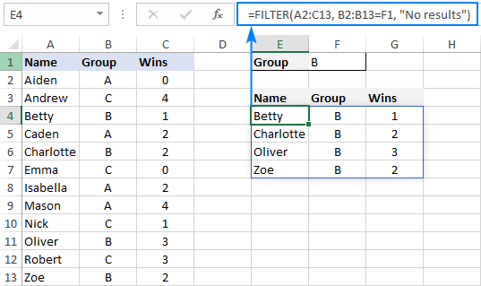
If no records match the specified criteria, the formula returns the value you put in the if_empty argument, "No results" in this example:
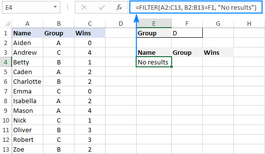
If you'd rather return nothing in this case, then supply an empty string ("") for the last argument:
=FILTER(A2:C13, B2:B13=F1, "")
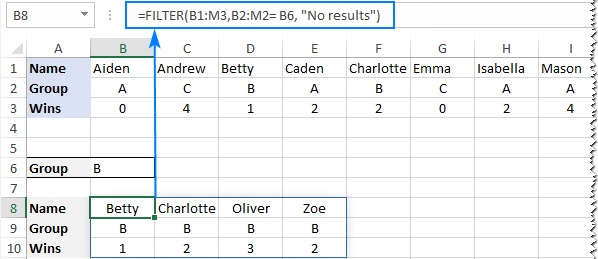
In case your data is organized horizontally from left to right like shown in the screenshot below, the FILTER function will work nicely too. Just make sure you define appropriate ranges for the array and include arguments, so that the source array and Boolean array have the same width:
=FILTER(B2:M4, B3:M3= B7, "No results")
Excel FILTER function - usage notes
To effectively filter in Excel with formulas, here are a couple of important points to take notice of:
- The FILTER function automatically spills the results vertically or horizontally in the worksheet, depending on how your original data is organized. So, please make sure you always have enough empty cells down and to the right, otherwise you'll get a #SPILL error.
- The results of the Excel FILTER function are dynamic, meaning they update automatically when values in the original data set change. However, the range supplied for the array argument is not updated when new entries are added to the source data. If you wish the array to resize automatically, then convert it to an Excel table and build formulas with structured references, or create a dynamic named range.
How to filter in Excel - formula examples
Now that you know how a basic Excel filter formula works, it's time to get some insights into how it could be extended for solving more complex tasks.
Filter with multiple criteria (AND logic)
To filter data with multiple criteria, you supply two or more logical expressions for the include argument:
The multiplication operation processes the arrays with the AND logic, ensuring that only the records that meet all the criteria are returned. Technically, it works this way:
The result of each logical expression is an array of Boolean values, where TRUE equates to 1 and FALSE to 0. Then, the elements of all the arrays in the same positions are multiplied. Since multiplying by zero always gives zero, only the items for which all the criteria are TRUE get into the resulting array, and consequently only those items are extracted.
The below examples show this generic formula in action.
Example 1. Filter multiple columns in Excel
Extending our basic Excel FILTER formula a little further, let's filter the data by two columns: Group (column B) and Wins (column C).
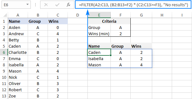
For this, we set up the following criteria: type the name of the target group in F2 (criteria1) and the minimum required number of wins in F3 (criteria2).
Given that our source data is in A2:C13 (array), groups are in B2:B13 (range1) and wins are in C2:C13 (range2), the formula takes this form:
=FILTER(A2:C13, (B2:B13=F2) * (C2:C13>=F3), "No results")
As the result, you get a list of players in group A who have secured 2 or more wins:
Example 2. Filter data between dates
First off, it should be noted that it's not possible to make up a generic formula to filter by date in Excel. In different situations, you will need to build criteria differently, depending on whether you want to filter by a specific date, by month, or by year. The purpose of this example is to demonstrate the general approach.
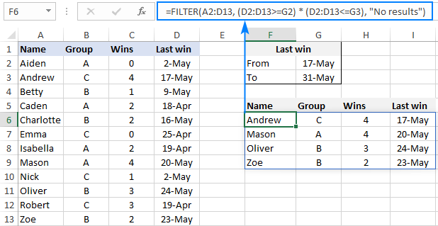
To our sample data, we add one more column containing the dates of the last win (column D). And now, we will extract the wins that occurred in a specific period, say between May 17 and May 31.
Please notice that in this case, both criteria apply to the same range:
=FILTER(A2:D13, (D2:D13>=G2) * (D2:D13<=G3), "No results")
Where G2 and G3 are the dates to filter between.
Filter with multiple criteria (OR logic)
To extract data based on multiple OR condition, you also use logical expressions like shown in the previous examples, but instead of multiplying, you add them up. When the Boolean arrays returned by the expressions are summed, the resulting array will have 0 for entries that do not meet any criteria (i.e. all the criteria are FALSE), and such entries will be filtered out. The entries for which at least one criterion is TRUE will be extracted.
Here's the generic formula to filter columns with the OR logic:
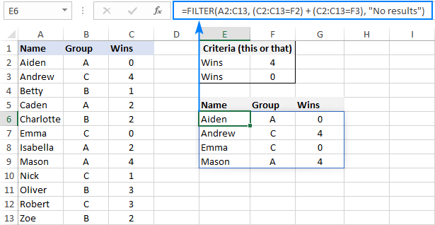
As an example, let's extract a list of players that have this or that number of wins.
Assuming the source data is in A2:C13, wins are in C2:C13, and the win numbers of interest are in F2 and F3, the formula would go as follows:
=FILTER(A2:C13, (C2:C13=F2) + (C2:C13=F3), "No results")
As the result, you know which players have won all the games (4) and which have won none (0):
Filter based on multiple AND as well as OR criteria
In situation when you need to apply both criteria types, remember this simple rule: join the AND criteria with asterisk (*) and OR criteria with the plus sign (+).
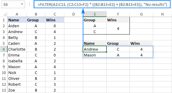
For example, to return a list of players that have a given number of wins (F2) AND belong to the group mentioned in either E2 OR E3, build the following chain of logical expressions:
=FILTER(A2:C13, (C2:C13=F2) * ((B2:B13=E2) + (B2:B13=E3)), "No results")
And you will get the following result:
How to filter duplicates in Excel
When working with huge worksheets or combining data from different sources, there's often a possibility that some duplicates would sneak in.
If you are looking to filter out duplicates and extract unique items, then use the UNIQUE function as explained in the above linked tutorial.
If your goal is to filter duplicates, i.e. extract entries that occur more than once, then use the FILTER function together with COUNTIFS.
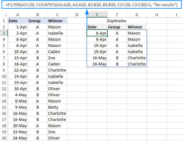
The idea is to get the occurrences counts for all the records and extract those greater than 1. To get the counts, you supply the same range for each criteria_range / criteria pair of COUNTIFS like this:
For example, to filter duplicate rows from the data in A2:C20 based on the values in all 3 columns, here's the formula to use:
=FILTER(A2:C20, COUNTIFS(A2:A20, A2:A20, B2:B20, B2:B20, C2:C20, C2:C20)>1, "No results")
Tip. To filter duplicates based on the values in the key columns, include only those specific columns in the COUNTIFS function.
How to filter out blanks in Excel
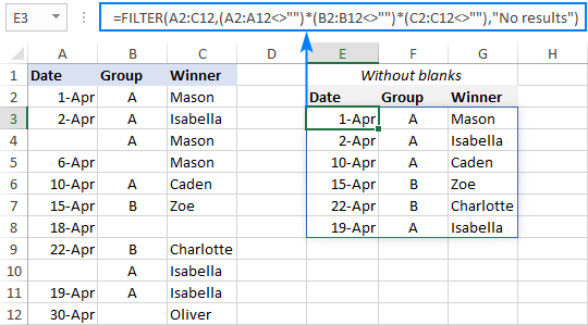
A formula for filtering out blank cells is, in fact, a variation of the Excel FILTER formula with multiple AND criteria. In this case, we check whether all (or particular) columns have any data in them and exclude the rows where at least one cell is empty. To identify non-blank cells, you use the "not equal to" operator (<>) together with an empty string ("") like this:
With the source data in A2:C12, to filter out rows containing one or more blank cells, the following formula is entered in E3:
Filter cells containing specific text
To extract cells that contain certain text, you can use the FILTER function together with the classic If cell contains formula:
Here's how it works:
- The SEARCH function looks for a specified text string in a given range and returns either a number (the position of the first character) or #VALUE! error (text not found).
- The ISNUMBER function converts all the numbers to TRUE and errors to FALSE and passes the resulting Boolean array to the include argument of the FILTER function.
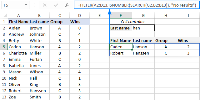
For this example, we've added the Last names of players in B2:B13, typed the part of the name we want to find in G2, and then use the following formula to filter the data:
=FILTER(A2:D13, ISNUMBER(SEARCH(G2, B2:B13)), "No results")
As the result, the formula retrieves the two surnames containing "han":
Filter and calculate (Sum, Average, Min, Max, etc.)
A cool thing about the Excel FILTER function is that it can not only extract values with conditions, but also summarize the filtered data. For this, combine FILTER with aggregation functions such as SUM, AVERAGE, COUNT, MAX or MIN.
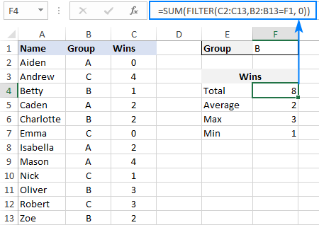
For instance, to aggregate data for a specific group in F1, use the following formulas:
Total wins:
=SUM(FILTER(C2:C13, B2:B13=F1, 0))
Average wins:
=AVERAGE(FILTER(C2:C13, B2:B13=F1, 0))
Maximum wins:
=MAX(FILTER(C2:C13, B2:B13=F1, 0))
Minimum wins:
=MIN(FILTER(C2:C13, B2:B13=F1, 0))
Please pay attention that, in all the formulas, we use zero for the if_empty argument, so the formulas would return 0 if no values meeting the criteria are found. Supplying any text such as “No results” would result in a #VALUE error, which is obviously the last thing you want :)
Case-sensitive FILTER formula
A standard Excel FILTER formula is case-insensitive, meaning it makes no distinction between lowercase and uppercase characters. To distinguish text case, nest the EXACT function in the include argument. This will force FILTER to do logical test in a case-sensitive manner:
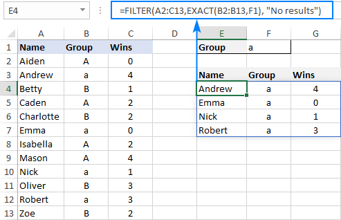
Supposing, you have both groups A and a and wish to extract records where the group is the lowercase "a". To have it done, use the following formula, where A2:C13 is the source data and B2:B13 are groups to filter:
=FILTER(A2:C13, EXACT(B2:B13, "a"), "No results")
As usual, you can input the target group in a predefined cell, say F1, and use that cell reference instead of hardcoded text:
=FILTER(A2:C13, EXACT(B2:B13, F1), "No results")
How to FILTER data and return only specific columns
For the most part, filtering all columns with a single formula is what Excel users want. But if your source table contains tens or even hundreds of columns, you may certainly want to limit the results to a few most important ones.
Example 1. Filter some adjacent columns
In situation when you want some neighboring columns to appear in a FILTER result, include only those columns in array because it is this argument that determines which columns to return.
In the basic FILTER formula example, supposing you wish to return the first 2 columns (Name and Group). So, you supply A2:B13 for the array argument:
=FILTER(A2:B13, B2:B13=F1, "No results")
As the result, we get a list of participants of the target group defined in F1:

Example 2. Filter non-adjacent columns
To cause the FILTER function to return non-contiguous columns, use this clever trick:
- Make a FILTER formula with the desired condition(s) using the entire table for array.
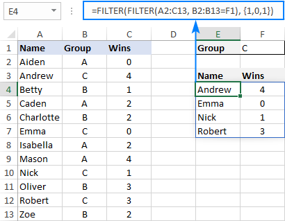
- Nest the above formula inside another FILTER function. To configure the "wrapper" function, use an array constant of TRUE and FALSE values or 1's and 0's for the include argument, where TRUE (1) marks the columns to be kept and FALSE (0) marks the columns to be excluded.
For example, to return only Names (1st column) and Wins (3rd column), we are using {1,0,1} or {TRUE,FALSE,TRUE} for the include argument of the outer FILTER function:
=FILTER(FILTER(A2:C13, B2:B13=F1), {1,0,1})
Or
=FILTER(FILTER(A2:C13, B2:B13=F1), {TRUE,FALSE,TRUE})
How to limit the number of rows returned by FILTER function
If your FILTER formula finds quite a lot of results, but your worksheet has limited space and you cannot delete the data below, then you can limit the number of rows the FILTER function returns.
Let's see how it works on an example of a simple formula that pulls players from the target group in F1:
=FILTER(A2:C13, B2:B13=F1)
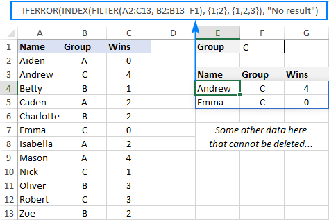
The above formula outputs all the records that it finds, 4 rows in our case. But suppose you just have space for two. To output only the first 2 found rows, this is what you need to do:
- Plug the FILTER formula into the array argument of the INDEX function.
- For the row_num argument of INDEX, use a vertical array constant like {1;2}. It determines how many rows to return (2 in our case).
- For the column_num argument, use a horizontal array constant like {1,2,3}. It specifies which columns to return (the first 3 columns in this example).
- To take care of possible errors when no data matching your criteria is found, you can wrap your formula in the IFERROR function.
The complete formula takes this form:
=IFERROR(INDEX(FILTER(A2:C13, B2:B13=F1), {1;2}, {1,2,3}), "No result")
When working with large tables, writing array constants manually may be quite cumbersome. No problem, the SEQUENCE function can generate the sequential numbers for you automatically:
=IFERROR(INDEX(FILTER(A2:C13, B2:B13=F1), SEQUENCE(2), SEQUENCE(1, COLUMNS(A2:C13))), "No result")
The first SEQUENCE generates a vertical array containing as many sequential numbers as specified in the first (and only) argument. The second SEQUENCE uses the COLUMNS function to count the number of columns in the dataset and produces an equivalent horizontal array.
Tip. To return data from specific columns, not all the columns, in the horizontal array constant that you use for the column_num argument of INDEX, include only those specific numbers. For instance, to extract data from the 1st and 3rd columns, use {1,3}.
Excel FILTER function not working
In situation when your Excel FILTER formula results in an error, most likely that will be one of the following:
#CALC! error
Occurs if the optional if_empty argument is omitted, and no results meeting the criteria are found. The reason is that currently Excel does not support empty arrays. To prevent such errors, be sure to always define the if_empty value in your formulas.
#VALUE error
Occurs when the array and include argument have incompatible dimensions.
#N/A, #VALUE, etc.
Different errors may occur if some value in the include argument is an error or cannot be converted to a Boolean value.
#NAME error
Occurs when trying to use FILTER in an older version of Excel. Please remember that it is a new function, which is only available in Office 365 and Excel 2021.
In new Excel, a #NAME error occurs if you accidentally misspell the function's name.
#SPILL error
Most often, this error occurs if one or more cells in the spill range are not completely blank. To fix it, just clear or delete non-empty cells. To investigate and resolve other cases, please see #SPILL! error in Excel: what it means and how to fix.
#REF! error
Occurs when a FILTER formula is used between different workbooks, and the source workbook is closed.
That's how to filer data in Excel dynamically. I thank you for reading and hope to see you on our blog next week!
Download practice workbook
Filter in Excel with formulas (.xlsx file)
 by
by
349 comments
Your post on how to use excel filter function with multiple criteria was very helpful. Thank you for posting it.
I do have one situation that is not accounted for and hope it is something you could help with.
What if one of the cells that you are looking for a match in contains data on multiple lines. I want to be able to account for that and have the result return.
For example if in Cell B2 I have Nuts [carriage return] bolts, if I am looking for nuts I want the filter function to return data in that row.
Hi! If I understand correctly, you can use a partial match in the conditions of the FILTER function. You can use this guide: How to find substring in Excel. For example:
=FILTER(A2:B10,ISNUMBER(SEARCH("Nuts",B2:B10)))
Hiya
i have a formula =COUNTA(UNIQUE(FILTER('Data List'!C41974:C54033,'Data List'!A41974:A54033=Dashboard!B10))) however i need to base this formula on a year.
the spreadsheet list contains 10 of thousands lines including document name customer name qty and year.
i am trying to calculator the number of unique clients for a specific document name for a specific year
Hi! We have a special tutorial that can help to solve your problem: Count unique values with multiple criteria. I can't recommend a formula to you as I don't have an accurate description of your data.
good knowledge how to using the filter function.
Using {1,0,1} or {TRUE,FALSE,TRUE} for the include argument of the outer FILTER function to filter non-adjacent columns
works very well on a range of data. Still, it always displays those columns with zero values after converting the range to a Table. Is it a way to completely exclude those columns from showing up? Thanks.
Hello Julian!
If I understand your task correctly, add another condition to the FILTER function to exclude zero values. For example:
=IFERROR(INDEX(FILTER(A2:C13, (B2:B13=F1)*(C2:C13>0)), {1;2}, {1,2,3}), "No result")
After revisiting your sample file, I found a new function, CHOOSECOLS, that can be applied to choose the required columns as I mentioned. Thanks very much for your reply.
Great article. I am trying to figure out how to apply conditional formatting for all entries the FILTER function will be picking up considering it has to be dynamic as the data source will be changing. Any hints? Thanks!
Hello Armando!
To apply conditional formatting dynamically to the results of the Excel FILTER function, you can follow these steps:
Set Up Your Data and FILTER Function:
Assume your data is in the range A1:D10.
Use the FILTER function to extract data based on criteria. For example:
=FILTER(A1:D10, B1:B10="Criteria")
Apply Conditional Formatting:
Select the range where the FILTER function outputs its results.
Go to the Home tab, click on Conditional Formatting, and choose New Rule.
Select Use a formula to determine which cells to format.
Enter a formula that references the first cell of your FILTER output. For example, if your FILTER output starts at F1, you might use:
=F1>100
Set the formatting options you want (e.g., fill color, font color). Read more: Excel Conditional Formatting tutorial with examples.
Ensure Dynamic Range:
To make sure the conditional formatting applies dynamically as the FILTER function updates, use a formula that covers the entire range of potential output. For example:
=F1:F100>100
Modify the formula and formatting rules based on your specific criteria and data structure.
This approach ensures that as your data changes and the FILTER function updates its output, the conditional formatting will automatically apply to the new results.
Dear Sir,
I am using Excel 2016 i dont have option =Filtter, Please provide Module VBA Code
Hi,
I’m having trouble creating a filter formula that would populate sheets based on car brand and a drop down column. The goal is every time a drop down selection is made, the row of information will automatically populate into its respective sheet.
Below is breakdown:
Sheet1 is Masterlist which contains all information of cars : Honda, Nissan, Toyota, Lexus. Column B is name of brand and Column P ( drop down selection) would be status. The goal would anytime a new line is added with car brand, the information should only populate over into the other sheet once Column P has a status selected. The 3 statuses in the drop-down would be New,Old, Terminated.
An example of Honda Sheet would look like this
=Filter(‘Mastersheet’!B:R,(Mastersheet’!P:P=“New”)*(Masterlist’!B:B=“Honda”)+(Mastersheet’!P:P=“Old”)*(Masterlist’!B:B=“Honda”)+(Mastersheet’!P:P=“Terminated”)*(Masterlist’!B:B=“Honda”)
The formula seems to work when adjusting existing car statues in the Mastersheet. The lines disappear when I change the status to blank. However it won’t work when adding new lines to the list and changing the status.
Hello Joseph!
I don't really understand what your problem is. The formula will work when adding new records to the worksheet, as it references the entire column. When you change the status, the formula also works and changes the filter.
Thank you for responding!
It appears it stops working properly once the file becomes shared. Curly braces
are added to the formulas and it stops working the way it should be. After unsharing and eliminating the curly brackets, the formula works fine. Is there a way to eliminate the curly braces from being automatically added to the formulas after the file becomes shared?
Thank you for your help!
Hi! I’m having trouble creating a filter formula for the information below:
I want to filter information from Name And Serial#
I created multiple sheets which would populate the separate names and serial#s. They would all pull from the master sheet.
Below is my formula
=Filter(‘Mastersheet!’C:R,(Mastersheet!B:B=‘’Bob’’)*(Bob!A:A=“Bob”)*(‘Mastersheet!P:P=“Active”)
What I would like to do is anytime we receive a new serial number in the Mastersheet, I would paste the information into the person’s name sheet. I would like paste the name and serial number into column A and B in Bob’s sheet and populate the associated information of the serial number into columns C:R.
The formula above works to populate Bob but at times doesn’t correctly match the serial number. I’m thinking it would be a combo of match w/filter or xlookup w/ Filter
I know it can work with with a xlookup standalone but I don’t want to drag down the formula or keep the formula hidden in the blank cells. Thank you for your help!
To add for clarity
Mastersheet Column B - Name
Mastersheet Column C - Serial Number
In Bob sheet, I want to populate Data in columns C:R. Column A (Name -Bob) and Column B ( Serial Number associated with Bob) I would copy/paste into it. I guess what I want is the data associated with that specific serial number to populate automatically every time I paste name and serial number into column A and B without having to drag the formula down Ala xlookup
Hello Leonard!
I’m sorry, but your description doesn’t give me a complete understanding of your task. In your FILTER formula, you are using a condition on values from two worksheets. This will not work. In addition, they are writing that they want to filter information by serial number (column C). However, the serial number is not included in the conditions of your formula.
Without having an example of your data and desired result, I can't offer you a formula.
I currently use the transpose(filter) formula but need to do it to two separate arrays but both sets of data to come out of the same formula.
is there any way to do this
for example
A B C D
1 ge 4 ge
5 fr 7 fr
3 ge 6 fr
I would need to find the numbers corresponding with "ge" across the two different ranges but to be combined in the one filter
I hope this makes sense.
TIA
Hi! Unfortunately, your question is not quite clear. Write what result you wanted to get from your data.
Col a&b is one table and col c&d is another. I need to filter the results depending on the letters but want them to be combined
So for example the result for ge would be
1
3
4
Hi! Use the VSTACK function to create an array of 2 columns of data. You can select any column from this array using the CHOOSECOLS function. Use the FILTER function to get the data that matches the condition from the first column. Based on the information given, the formula could be as follows:
=FILTER(CHOOSECOLS(VSTACK(A1:B4,C1:D4),1), CHOOSECOLS(VSTACK(A1:B4,C1:D4),2)="ge")
I hope it’ll be helpful.
I tried the formula you gave. It is only giving the first instance and no other. So it is only giving one result.
Hi! I used this formula for your data and got exactly the three numbers you specified. Perhaps these functions are not available in your version of Excel. Describe the problem and the result in more detail.
The data I gave is just an example of what I am looking at. There is more of the same information in the columns and gaps also. Only the first instance is given in the filter result.
I am unsure but believe the version is Excel365 and the workbook is a shared workbook.
Hi! In Excel365 on your data using this formula I got 3 results. Read carefully the articles I recommended and you will understand how the formulas work and solve the problem.
I have a document that uses the filter to copy text from one tab to another. However if the original tab has over 40 words the copied location just shows 0. anything under 40 words copies fine. Any idea
Hi! I can't see your data and I don't know what formula you are using. Therefore, I cannot say anything about the cause of the problem. Excel difficulties may be due to insufficient computer RAM.
When I put the file in share, the filter does not work anymore... Is there a way to change that or is it normal ?
Hello! It’s a common issue that filters may not work as expected in shared Excel files. When a workbook is shared, certain features, like Auto Filter, Advanced Filter, and some sorting and filtering options, can behave differently or may not be available.
The reason could be Excel Online Limitations: Some advanced filtering features available in the Excel desktop app might not be fully supported in Excel Online.
Here are a few steps you can try to resolve the filter issue:
Select All Data: Ensure your table doesn’t have blank rows or columns that might prevent the filter from selecting the entire area.
Remove Blank Rows/Columns: Configuring the data in your Filter area to remove blanks can help.
Unhide Rows/Columns: Hidden rows or columns can interfere with filtering.
Unmerge Cells: Merged cells can cause issues with filtering.
Clear and Reapply Filter: Sometimes, simply clearing the existing filter and applying it again can fix the issue.
The FILTER function works perfectly fine for me. Because my data is in a row, it's returning the results in a row. Is it possible display the results in a column?
My filter results are currently displaying as:
Row 1: Apple, Pears, Bananas
I want it to display as follows:
Column A
Apple
Pears
Bananas
Thanks.
I've worked it out! TRANSPOSE was the function I was looking for.
Great website, it's helped me a lot with the spreadsheet I'm currently working with.
Hi! Here is the article that may be helpful to you: Excel TRANSPOSE function to change columns to rows.
Hmm, was hoping the “How to filter out blank cells” would work, I’m trying to just copy data and “hide” the zero values…I'm pulling data for a 3D pie chart and the 3D pie chart as far as I know doesn't have a function to eliminate the zeros from the chart legend. In other words my data looks like this:
Column A / Column B
A / 50
B / 100
C / 75
D / 25
Other / 50
So with my pie chart as long as all 4 options are filled in (A through D), then my chart works great. However, since I'm pulling data, if less than 4 are fill out it leaves a blank line:
Column A / Column B
A / 50
B / 100
Other / 0
In other words, the pie chart is pulling from A through "Other" and where C and D would be it's now entering 0s into the legend of the pie chart. ("Other" is actually pulling additonal data that goes further than 4 and combining it all)
What I want to do is copy this data into 2 new columns so I can just pull my pie chart from that.
The end product I'm looking for would be:
Column A / Column B
A / 50
B / 100
Other / 0
This way the 3rd and 4th rows that are blank wouldn't show up and the data below would be pushed up (I wouldn't mind hiding the "Other" as well since it will show 0 but that isn't necessary.
Anyways, hope this makes sense. Any help at all would be appreciated. TIA.
Hi! To extract all non-empty rows from a range in Excel, you can use the FILTER function with BYROW function. Here is an example formula that allows you to do this:
=FILTER(A1:B7, BYROW(A1:B7, LAMBDA(row, SUM(--(row<>""))>0)))
This formula uses the LAMBDA function to check each row for non-empty cells and only returns rows where the sum of non-empty cells is greater than zero.
Make sure you have the latest version of Excel installed, as the FILTER and LAMBDA function is available starting with Excel 365.
You can also solve your problem with a VBA macro.
Hey thank you! This worked on 3/4 tabs. Unsure as to why the one isn't working as I've checked multiple times and I did the exact same thing...hmm. Maybe I'll start back from scratch on that one...either way it looks promising. Thanks again.
Very illustrative the use of the FILTER function, but unfortunately, I couldn't find any good explanation about how to include and exclude at the same time some matchings. For example, you mentioned how to filter some matches containing some words:
FILTER(array, ISNUMBER(SEARCH("text", range)), "No results")
but what about if I want to filter out some results that contain some words?
And ultimately, how to filter in and filter out a table that contains or does not contain some words??
🤷♂️
Hi! To filter out results that contain some words, use this paragraph in the article above: Filter with multiple AND criteria.
To filter out data that does not contain a certain word, add the NOT function to the recommended formulas above. For example:
=FILTER(A2:D13, NOT(ISNUMBER(SEARCH(G2, B2:B13))), "No results")
I hope it’ll be helpful. If something is still unclear, please feel free to ask.
Hi. how to install filter and colcolumn function? Does it work office 2019?
Hi! Read the article above carefully. The FILTER function is not supported in Excel2019.
I have this data where, collumn 1 is stock names, collumn 2 is activity of stock (Buy/Sell) meaning some stock were sold or bought, collumn 3; I want to create collumn 3, such that it picks the name of the stock in collumn 1, if there is no balance of stock remaining in collumn 2, how do i go about this?
Remember the stocks are bought and sold in different dates. Will appreciate any help.
Hi! I can't see your data, but I can guess that if a stock was bought and then sold, it is written twice in column A. If you select unique values from column A, it will be a list of stock remaining. Look for the example formulas here: Excel UNIQUE function - fastest way to find unique values. If I'm not guessing, give me an example of source data and the desired result.
Hello Alex.
Also its good to say that, I am using excel 2019, so the UNIQUE function and FILTER functions are not working.
Regards.
Hello Alex.
Thank you very much for your reply. Here is a sample data of the table: The collumn 1; is Name of Stock. Collumn 2: Transaction, Collumn 3: Date of the Transaction. Collumn 4: Quantity.....You will notice some stocks were fully sold out. So, we only want to have a new collumn 4, which is only picking the Name of the stock with a positive value and omit out the stock that has been sold out.
STOCK: TRANSACTION: DATE: QUANTITY:
Amazon $$$: Buy: 1/30/2023; 70
Costco Wholesale $$$ : Buy: 2/5/2023: 25
Enphase $$$: Buy: 2/12/2023: 30
T- Mobile $$$: Buy: 2/19/2023: 1000
Wells Fargo $$$: Buy: 2/26/2023: 40
Amazon $$$: Sell: 3/19/2023: -45
Costco Wholesale $$$: Sell: 4/9/2023: -25
Enphase $$$: Sell: 4/16/2023: -25
T- Mobile $$$: Sell: 4/23/2023: -15
Wells Fargo $$$: Sell: 5/14/2023: -40
Then the expected outcome will be a collumn only showing the stocks with a balance, and it should not leave or show empty cells:
STOCK:
Amazon $$$:
Enphase $$$:
T- Mobile $$$:
If you can share a formula that will work this out, I will be forever greatful.
Kind Regards.
Hi! To get a table of stocks with balance, you can create a pivot table. Using the SUMIFS formula, you can calculate the balance for each individual stock. For example,
=SUMIFS(C1:C10,A1:A10,"Amazon $$$",B1:B10,"Buy") - SUMIFS(C1:C10,A1:A10,"Amazon $$$",B1:B10,"Sell")
I recommend reading this guide: Excel SUMIFS and SUMIF with multiple criteria – formula examples.
Thanks Alex.
I have tried that formula it still gives wrong answers. I mean i want the formula that will give a collumn that picks the name of the stock which has positive balance of stock, and ignore and omit out completely those stock that have zero balance.
Will appreciate.
The formula works with the data you gave. In your Excel2019 there are no other options other than what I have written to you.
Hello Alex, sorry i made a slight typing error above:
i have this scenario: Collumn 1 has names of stock, collumn 2 has price of stock. collumn 3 has new names of stock. I am looking a formula which looks for names in collumn 3 and matches them against names in collumn 1, if the name is identified, we pick the price indicated in collumn 2. I tried this formula, but i realised it picks some prices correctly while others it gives a wrong answer, kindly confirm if there is something i am missing from this formula:
=FILTER('Collumn 2'!B2:B125, COUNTIF(Collumn 3!B2:B125, 'Collumn 1'!A2:A125) > 0)
Unfortunately, without seeing your data it is difficult to give you any advice. Please provide me with an example of the source data and the expected result.
Hello Alex,
Again, i have this scenario: Collumn 1 has names of stock, collumn 2 has price of stock. collumn 3 has new prices of stock. I am looking a formula which looks for names in collumn 3 and matches them against names in collumn 1, if the name is identified, we pick the price indicated in collumn 2. I tried this formula, but i realised it picks some prices correctly while others it gives a wrong answer, kindly confirm if there is something i am missing from this formula:
=FILTER('Collumn 2'!B2:B125, COUNTIF(Collumn 3!B2:B125, 'Collumn 1'!A2:A125) > 0)
Will appreciate your help.
Regards.
Hi! What is written in column 3 - new prices or names? I don't have your data, so I can't understand or check your formula. I can't guess which result you want.
Hello Alex.
Thank you for the guide, It finally worked fine after fine tuning the formula.
I appreciate big time.
Thanks Alex.
I followed the given page and formula. this is the formula i used:
=IF(SUMIFS(E:E, B:B, B2) > 0, B2, "") this was able to give me a collumn with values which are positive.
this is what result i got:
Metta $$
Amazon $$$
Costco Wholesale $$$
Enphase $$$
T- Mobile $$$
Wells Fargo $$$
Amazon $$$
Is there a formula i can use such that, it will skip these empty cells and pick the others?
Regards.
Maybe this guide will be helpful: Extract a list of data ignoring blank cells.
Thanks Alex for the reply.
However i have gone through the page and made adjustments accordingly to map the cells and ranges correctly,but i noticed, its giving the answer as a value. But i am looking for the answer to be the NAME OF STOCK.
Pardon for asking, will appreciate your guide kindly.
Hi! In your version of Excel, you can calculate the balance for each stock in a separate column and then use Advanced Filter to select a unique list of stocks with positive balances. Read more: Excel Advanced Filter - how to create and use.
Or instead of Advanced Filter, you can use these instructions: Find unique and distinct rows.
In newer versions of Excel, this can be done with a single formula using the FILTER and UNIQUE functions as described in this guide: Filter unique values based on multiple criteria.
Thanks Alex.
When i paste the formula to the collumn of the same table i shared, it gives me these values which are not correct. Kindly check it out, I might be missing out on something, kindly guide
-48
-48
-45004
-45004
-45004
-45004
-45004
0
0
0
while i am looking for an output with only NAME OF STOCK which happens to have a balance value greater than zero.
Will appreciate your help.
Note that the formula is given to you for an example. I have no way of knowing what columns your data is in. Study the guide to the SUMIFS function that I recommended. If necessary, change the data references in the formula. I can help, but not do your work for you.
Can wildcards be used as filter criteria?
Pay attention to the following paragraph of the article above: Filter cells containing specific text.
I have the problem that I want to use a dynamic criteria range also in filter function, but it didn't work.
formular works by its own, but I don't want to duplicate formular with copy paste, because column count changes
my idea works fine, on substraction or sumifs like:
=IFERROR(+(B3:OFFSET(B3;0;ROWS(select_prj#)-1))-(B19:OFFSET(B19;0;ROWS(select_prj#)-1));"") where select_prj# = range of elements I want to work with
also works fine:
=UNIQUE(FILTER(Einzelposten_ab_2019!S:S;(Einzelposten_ab_2019!A:A=B3)*(Einzelposten_ab_2019!AH:AH="Rev")))
but combined I get an error
I tried:
=UNIQUE(FILTER(Einzelposten_ab_2019!S:S;(Einzelposten_ab_2019!A:A=(B3:OFFSET(B3;0;ROWS(select_prj#)-1)))*(Einzelposten_ab_2019!AH:AH="Rev")))
any idea how to solve?
Hi! I don't have your data, so I can't understand or check your formula. I can't guess which result you want. Please clarify your specific problem or provide additional information to understand what you need.
I want to use filter, but my 'Include' is a formula that looks at the current time of day, when it do that nothing shows up, however if i type a fixed date, rather than the formula it works?
Hi! Unfortunately, I can't see your data and can't guess what formula you are using.
Hi, I want to use something like this: =FILTER(B57:M3041,ISNUMBER(SEARCH(P1:P52,J57:J3041))=FALSE) to filter a list. I want it to NOT contain any of the values in a list (P1:P52), but it only seems to be looking at the first one in the list (P1) and filtering that. How can I do this with a list of 52 things I want to filter out? Thanks!