The tutorial shows how you can leverage the new SEQUENCE function to quickly generate a list of dates in Excel and use the AutoFill feature to fill a column with dates, workdays, months or years.
Until recently, there has been just one easy way to generate dates in Excel - the AutoFill feature. The introduction of the new dynamic array SEQUENCE function has made it possible to make a series of dates with a formula too. This tutorial takes an in-depth look at both methods so that you can choose the one that works best for you.
How to fill date series in Excel
When you need to fill a column with dates in Excel, the fastest way is to use the AutoFill feature.
Auto fill a date series in Excel
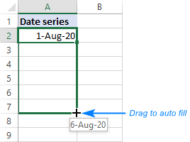
Filling a column or row with dates that increment by one day is very easy:
- Type the initial date in the first cell.
- Select the cell with the initial date and drag the fill handle (a small green square at the bottom-right corner) down or to the right.
Excel will immediately generate a series of dates in the same format as the first date that you typed manually.
Fill a column with weekdays, months or years
To create a series of workdays, months or years, do one of the following:
- Fill a column with sequential dates as described above. After that, click the AutoFill Optionsbutton and pick the desired option, say Fill Months:
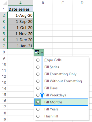
- Or you can enter your first date, right-click the fill handle, hold and drag through as many cells as needed. When you release the mouse button, a context menu will pop-up letting you select the needed option, Fill Years in our case:

Fill a series of dates incrementing by N days
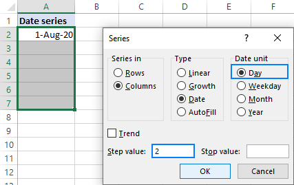
To auto generate a series of days, weekdays, months or years with a specific step, this is what you need to do:
- Enter the initial date in the first cell.
- Select that cell, right-click the fill handle, drag it through as many cells as needed, and then release.
- In the pop-up menu, choose Series (the last item).
- In the Series dialog box, select the Date unit of interest and set the Step value.
- Click OK.
For more examples, please see How to insert and autofill dates in Excel.
How to make a date sequence in Excel with a formula
In one of the previous tutorials, we looked at how to use the new dynamic array SEQUENCE function to generate a number sequence. Because internally in Excel dates are stored as serial numbers, the function can easily produce a date series too. All you have to do is to correctly configure the arguments as explained in the following examples.
Note. All the formulas discussed here only work in the latest versions of Excel 365 that support dynamic arrays. In pre-dynamic Excel 2019, Excel 2016 and Excel 2013, please use the AutoFill feature as shown in the first part of this tutorial.
Create a series of dates in Excel
To generate a sequence of dates in Excel, set up the following arguments of the SEQUENCE function:
- Rows - the number of rows to fill with dates.
- Columns - the number of columns to fill with dates.
- Start - the starting date in the format that Excel can understand, like "8/1/2020" or "1-Aug-2020". To avoid mistakes, you can supply the date by using the DATE function such as DATE(2020, 8, 1).
- Step - the increment for each subsequent date in a sequence.
For example, to make a list of 10 dates starting with August 1, 2020 and increasing by 1 day, the formula is:
=SEQUENCE(10, 1, "8/1/2020", 1)
or
=SEQUENCE(10, 1, DATE(2020, 8, 1), 1)
Alternatively, you can input the number of dates (B1), start date (B2) and step (B3) in predefined cells and reference those cells in your formula. Since we are generating a list, the columns number (1) is hardcoded:
=SEQUENCE(B1, 1, B2, B3)
Type the below formula in the topmost cell (A6 in our case), press the Enter key, and the results will spill across the specified number of rows and columns automatically.
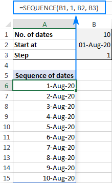
Note. With the default General format, the results will appear as serial numbers. To have them displayed correctly, be sure to apply the Date format to all the cells in the spill range.
Make a series of workdays in Excel
To get a series of working days only, wrap SEQUENCE in the WORKDAY or WORKDAY.INTL function this way:
As the WORKDAY function adds the number of days specified in the second argument to the start date, we subtract 1 from it to have the start date itself included in the results.
For instance, to generate a sequence of workdays starting on the date in B2, the formula is:
=WORKDAY(B2-1, SEQUENCE(B1))
Where B1 is the sequence size.

Tips and notes:
- If a start date is Saturday or Sunday, the series will begin on the next working day.
- The Excel WORKDAY function assumes Saturday and Sunday to be weekends. To configure custom weekends and holidays, use the WORKDAY.INTL function instead.
Generate a month sequence in Excel
To create a series of dates incremented by one month, you can use this generic formula:
In this case, you put the target year in the 1st argument and day in the 3rd argument. For the 2nd argument, the SEQUENCE function returns sequential numbers from 1 to 12. Based on the above parameters, the DATE function produces a series of dates like shown in the left part of the screenshot below:
=DATE(2020, SEQUENCE(12), 1)
To display only the month names, set one of the below custom date formats for the spill range:
- mmm - short form like Jan, Feb, Mar, etc.
- mmmm - full form like January, February, March, etc.
As the result, only the month names will appear in cells, but the underlying values will still be full dates. In both series in the screenshot below, please notice the default right alignment typical for numbers and dates in Excel:

To generate a date sequence that increments by one month and starts with a specific date, use the SEQUENCE function together with EDATE:
The EDATE function returns a date that is the specified number of months before or after the start date. And the SEQUENCE function produces an array of 12 numbers (or as many as you specify) to force EDATE to move forward in one-month increments. Please notice that the start argument is set to 0, so that the start date gets included in the results.
With the start date in B1, the formula takes this shape:
=EDATE(B1, SEQUENCE(12, 1, 0))

Note. After completing a formula, please remember to apply an appropriate date format to the results for them to display correctly.
Create a year sequence in Excel
To make a series of dates incremented by year, use this generic formula:
Where n is the number of dates you want to generate.
In this case, the DATE(year, month, day) function constructs a date in this way:
- Year is returned by the SEQUENCE function that is configured to generate an n rows by 1 column array of numbers, starting at the year value from start_date.
- Month and day values are pulled directly from the start date.
For example, if you input the start date in B1, the following formula will output a series of 10 dates in one-year increments:
=DATE(SEQUENCE(10, 1, YEAR(B1)), MONTH(B1), DAY(B1))
After being formatted as dates, the results will look as follows:

Generate a times sequence in Excel
Because times are stored in Excel as decimals numbers representing a fraction of the day, the SEQUENCE function can work with times directly.
Assuming the start time is in B1, you can use one of the following formulas to produce a series of 10 times. The difference is only in the step argument. As there are 24 hours in a day, use 1/24 to increment by an hour, 1/48 to increment by 30 minutes, and so on.
30 minutes apart:
=SEQUENCE(10, 1, B1, 1/48)
1 hour apart:
=SEQUENCE(10, 1, B1, 1/24)
2 hours apart:
=SEQUENCE(10, 1, B1, 1/12)
The screenshot below shows the results:

If you do not want to bother calculating the step manually, you can define it by using the TIME function:
For this example, we'll input all the variables in separate cells like shown in the screenshot below. And then, you can use the below formula to generate a time series with any increment step size you specify in cells E2 (hours), E3 (minutes) and E4 (seconds):
=SEQUENCE(B2, B3, B4, TIME(E2, E3, E4))

How to create a monthly calendar in Excel
In this final example, we'll be using the SEQUENCE function together with DATEVALUE and WEEKDAY to create a monthly calendar that will update automatically based on the year and month that you specify.
The formula in A5 is as follows:
=SEQUENCE(6, 7, DATEVALUE("1/"&B2&"/"&B1) - WEEKDAY(DATEVALUE("1/"&B2&"/"&B1)) + 1, 1)
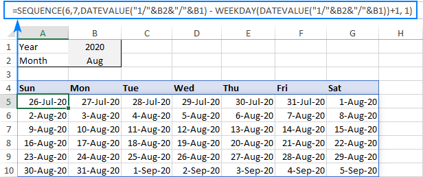
How this formula works:
You use the SEQUENCE function to generate a 6 rows (the max possible number of weeks in a month) by 7 columns (the number of days in a week) array of dates incremented by 1 day. Hence, the rows, columns and step arguments raise no questions.
The trickiest part in the start argument. We cannot start our calendar with the 1st day of the target month because we do not know which day of the week it is. So, we use the following formula to find the first Sunday before the 1st day of the specified month and year:
DATEVALUE("1/"&B2&"/"&B1) - WEEKDAY(DATEVALUE("1/"&B2&"/"&B1)) + 1
The first DATEVALUE function returns a serial number that, in the internal Excel system, represents the 1st day of the month in B2 and the year in B1. In our case, it's 44044 corresponding to August 1, 2020. At this point, we have:
44044 - WEEKDAY(DATEVALUE("1/"&B2&"/"&B1)) + 1
The WEEKDAY function returns the day of the week corresponding to the 1st day of the target month as a number from 1 (Sunday) to 7 (Saturday). In our case, it's 7 because August 1, 2020 is Saturday. And our formula reduces to:
44044 - 7 + 1
44044 - 7 is 4403, which corresponds to Saturday, July 25, 2020. As we need Sunday, we add the +1 correction.
This way, we get a simple formula that outputs an array of serial numbers beginning with 4404:
=SEQUENCE(6, 7, 4404, 1)
Format the results as dates, and you'll get a calendar shown in the screenshot above. For example, you can use one of the following date formats:
- d-mmm-yy to display dates like 1-Aug-20
- mmm d to display month and day like Aug 20
- d to display only the day
Wait, but we aim to create a monthly calendar. Why do some dates of the previous and next month show up? To hide away those irrelevant dates, set up a conditional formatting rule with the below formula and apply the white font color:
=MONTH(A5)<>MONTH(DATEVALUE($B$2 & "1"))
Where A5 is the leftmost cell of your calendar and B2 is the target month.

For the detailed steps, please see How to create a formula-based conditional formatting rule in Excel.
That's how you can generate a sequence of dates in Excel. I thank you for reading and hope to see you on our blog next week!
Practice workbook for download
Date sequence in Excel - formula examples (.xlsx file)
 by
by
211 comments
Is there a formula to automatically pull the following Mondays date in a cell? I have used =IF(A1 > 2, B1 + (8 - WEEKDAY(B1, 2)), B1) but that is pulling the closest Monday not the next Monday. I have an order form I send out that needs to have the next Mondays date.
Hi! Your question isn't very clear, as the formula B1 + 8 - WEEKDAY(B1, 2) retrieves the next Monday from the given date. Also, the result of your formula depends on the value of A1.
Hi! I wanted to create a formula that can generate a monthly schedule based on the start date at the top of the year (e.g., start date = 9/25/25 and schedule = 2nd Tuesday of every month). Thank you.
Hello Samantha!
Write the start date in A1 and try this formula
=EOMONTH($A$1,ROW(A1)-1)+1 + MOD(2 - WEEKDAY(EOMONTH($A$1,ROW(A1)-1)+1,2), 7) + 7
Use EOMONTH function to calculate the first day of a target month.
Function WEEKDAY returns the day of the week number (1=Monday, 2=Tuesday).
MOD(2 - WEEKDAY(...),7) — offset from the 1st day of the week to the first Tuesday (2 = Tuesday). Read more: Excel MOD function to get remainder.
+7 — converts the first Tuesday to the second.
You can copy this formula down along the column.
I am trying to create a yearly calendar, where 1-1-25 starts in the "2nd week" of 2025. I want to establish every 4 weeks and be able to change each year and it continue the pattern.
Hi! Unfortunately, this information is not enough to understand exactly what you need. For example, you can subtract a desired number of days from the current date to shift the calendar by that number of days. Read more: How to add and subtract dates in Excel. If this is not what you wanted, please describe the problem in more detail.
I am trying to get day and dates to be sequential in excel and be able to fill the cells down.
Tuesday August 5, 2025
Wednesday August 6, 2025
and so on including Sat and Sun
I am using Office 2019
Thanks
Hello Terry!
If the SEQUENCE function is not available to you, you can set the start date using DATE function and use this formula:
=CEILING(DATE(2025,8,4)+ROW(A1),1)
Set the date format you need in the cell with formula, as described in this instruction: How to change Excel date format and create custom formatting.
Copy formula down along the column.
Hello, I am trying to sequence a series of increasing dates across merged cells. I have Colum H7 and I7 merged together and Column H8 and I8 merged together, this pattern repeats itself across to DV & DW. I have my date, which is manually entered by me in Column B7 as the date I wish to start and I have the number of days in Column B8 as the duration I want the dates to cover, eg B7 = 12/03/2025 & B8= 7 then my date series would start on the 12/03/2025 and list the dates horizontally till the 18/03/2025. I have the following formula in cell H8 =SEQUENCE(1,B8,B7,1) and the following formula in Cell H7 dragged all the way across to cell DW =TEXT(H8,"ddd"). This lets me put a date in Cell B7 and a duration in cell B8 that then generates the dates in the form of dd/mm/yyyy in cell H8 increasing by 1 every next cell and the day in Cell H7 in the form of TUE increasing by one every next cell. The problem is the merged cells wont let me continue the formula and I get a spill error, is there a way to word the formula so it misses one column and continues the sequence in the column after, for example I put the formula in the merged H&I and it skips cell I and puts the next sequence date in the merged J&K and so on accross the sheet.
Hello Simon!
Unfortunately, in Excel, the dynamic array formula cannot correctly write values to the merged cells. Spill range cannot contain merged cells. Read more in this guide.
Looking at your "Generate a month sequence in Excel" formula: =DATE(YEAR(A3),SEQUENCE(12),1). Is there a way to alternate between two specific days of a month within the sequence ie.
12/15/24
1/1/25
1/15/24
2/1/25
2/15/25
etc.
Hello Brandon!
If I understand your task correctly, try the following formula:
=DATE(YEAR(A3), CEILING(SEQUENCE(24,1,1,1)/2,1), IF(MOD(SEQUENCE(24),2)=0,15,1))
The CEILING function helps to create a sequence of numbers in which each number is repeated twice. MOD function returns 0 for even numbers. You can also use the ISEVEN function:
=DATE(YEAR(A3), CEILING(SEQUENCE(24,1,1,1)/2,1), IF(ISEVEN(SEQUENCE(24)),15,1))
That does it!
I was working on =DATE(YEAR(A3),SEQUENCE(12),{1,15}), but it was giving me two side by side columns.
Thank you
Can you create 2 sequences in one cell? I need the following sequence of date and time to look like this in the same cell: 1/1/2026 6:05.
I tried =SEQUENCE(30,1,DATE(2024,11,1),2)*(SEQUENCE(30,1,TIME(10,11,0))) but it returns crazy dates like 1952, 2077 etc. I don't really care what the time is, it just has to be in there for the software. Can this be accomplished?
Thank-you!
Hello Teresa!
I don't know what results you want to get, but if you replace the multiplication sign with a "+" sign in the formula, you will get the date and time in the first cell. In the date format “dd/mm/yyyy hh:mm:ss” this is 01/11/2024 10:11:00
Hi, please help me to create formula for calendar (Sun to Sat) starting from 26th of each month and ends with 25th the next month. Eg: 26-aug to 25-sept. I don't know how to set the weekday return date in the sequence formula. Also, how was the rule formula for its conditional formatting to show only those dates. Thank you so much for this blog. It's really helpful.
Hi! You cannot create a date sequence using SEQUENCE function because each following month has a different number of days. Therefore, use WORKDAY.INTL function.
Set the start date in cell A1 and copy this formula down the column as far as necessary. Set the [weekend] argument and specify the weekend. If I understand your task correctly, try the following formula:
=WORKDAY.INTL($A$1,ROW(A1),1)
If this is not what you wanted, please describe the problem in more detail.
Thank you for replying but I want it in a calendar form. I am new to workday function. Therefore, I have this formula for my calendar;
=SEQUENCE(6, 7, DATEVALUE("26/"&A1&"/"&E1) - WEEKDAY(DATEVALUE("26/"&A1&"/"&E1)-1))
with: A1= months (in a dropdown), E1= years (in a dropdown). Looks like it's working but I just need to set the rules in conditional formatting something like =MONTH(A3)MONTH($A$1&$E$1)? to clear the font color for the dates shown on the calendar before 26th of the month, and after 25th next month. It is possible? If not, just have to manually do it. Or will the workday function solve it?
Hi! Your second question is different from the previous question because you were previously talking about weekdays. To modify the calendar formula that is described in paragraph: How to create a monthly calendar in Excel, try this formula:
=SEQUENCE(6,7,DATEVALUE("1/"&$B$2&"/"&$B$1)-6 - WEEKDAY(DATEVALUE("1/"&$B$2&"/"&$B$1)-6)+1, 1)
For conditional formatting of dates, use this formula:
=NOT((A5>=EDATE(DATEVALUE("1/"&$B$2&"/"&$B$1),-1)+25)*(A5<=DATEVALUE("1/"&$B$2&"/"&$B$1)+24))
I recommend reading this guide: Excel EDATE function to add or subtract months from date.
Hi! I apologize for not phrasing it correctly initially, but I meant the same thing. Oh my goodness, it works wonderfully, thank you so much!
Hi, is there an addition to the formula so I can exclude the timestamp? Even though I have changed the cell formatting, I am still getting a timestamp when I export my data.
This is my formula.
=SEQUENCE(6,7,DATEVALUE("1/"&B10&"/"&B9) - WEEKDAY(DATEVALUE("1/"&B10&"/"&B9))+1, 1)
Thank you!
Hello Emma!
Your formula returns a sequence of dates. Use the date format of your choice. Do not use time in these custom formats. The following tutorial should help: How to change Excel date format and create custom formatting.
Yes I am aware it is a sequence of dates which is what I need, however when I export the data, it gives me the date with a timestamp even though I have formatted the cell data to be a date format only.
Hi! You can convert your dates to text and then export them. For the detailed instructions, please see: Convert date to text in Excel - TEXT function and no-formula ways.
Hi,
I am looking to generate a schedule for customers, based on their choice of start dates and repeating on their choice of weekdays. ie as inputs we have a start date and possibly multiple days of week, say monday, wednesday and friday. A schedule is to be generated based on these for defined number of weeks, say 20.
can you help me with a formula for this in excel?
Hi! Use WORKDAY.INTL to exclude Sunday from the working days list. To increase the start date by 2 days as many times as required, use the SEQUENCE function to create a sequence of numbers in steps of 2. I believe the following formula will help you solve your task:
=WORKDAY.INTL(A1,SEQUENCE(60,1,0,2),11)
A1 - any Monday
Hi,
Thank you for the quick response.
The formula given is giving a schedule repeating after 2 working days rather than repeating the same 3 days of the week. Also, the days of the week needs to be customizable. ie some customers may opt only for monday, some for monday and wednesday and some for monday, wednesday and thursday etc. So this data will be available in another table, ie which days they have chosen. This input table can be amended to whatever format that helps in generating this schedule.
I may be asking for too much, but if this is possible it will greatly help
Thanks in advance
The formula I sent to you was created based on the description you provided in your first request. However, as far as I can see from your second comment, your task is now different from the original one.
With the [weekend] parameter of the WORKDAY.INTL function, you can set only the days of the week you need as working days. Then use the SEQUENCE function to sequentially add 1 day to the date.
For example, Monday and Wednesday:
=WORKDAY.INTL(A1,SEQUENCE(10,1,0,1),"0101111")
Thank you so much.
It worked perfectly with some minor modifications.
Apologise for the confusion. Probably I was not sufficiently clear in my communication.
Cheers!
Just to clarify, schedule is to be generated for each individual customer separately, based on their individual choice of days of the week
Hello.
I was looking for a formula where it formulates a date 5 years from the dates below. I need it to calculate the new date from 5 years of the dates below. I would need it to apply to a whole column as there is around 1000 rows. Thank you
4/7/2023
6/5/2024
7/31/18
2/17/17
11/2/04
Hi! Try to follow the recommendations from this article: How to subtract or add years to date in Excel. The formula might look like this:
=DATE(YEAR(A2) + SEQUENCE(10,1,5,5), MONTH(A2), DAY(A2))
Hello, I need to create a date sequence that only displays every Friday and Saturday Starting with Friday July 5, 2024, Saturday July 6, 2024 and ending with Friday June 27, 2025 and Saturday June 28, 2025.
Thank you in advance for any help on this.
Hello! Set the start date with the DATE function. Use the SEQUENCE function to create a 360-day date sequence. Use the WEEKDAY function to get the number of the day of the week. Use the FILTER function to get only Friday and Saturday.
=FILTER(DATE(2024,7,5)+SEQUENCE(360,1,0,1), WEEKDAY(DATE(2024,7,5)+SEQUENCE(360,1,0,1),15)<3)
Wow! Brilliant! May I ask if it is possible to include the day of the week in front of the date, and have the date displayed as follows: Friday July 5, 2024. The formula that you suggested displays in numeric format. Thank you again!!
Hi! Set the custom date format in the cells as described in these instructions: How to change Excel date format and create custom formatting. Here is an example of the date format code: dddd mmmm d, yyyy.
I figured it out!! Thank you so much for the guidance!
Hello Alexander,
I wasn't able to do it. Are you able to kindly show me in the formula how this is done?
To remind...you provided the formula =FILTER(DATE(2024,7,5)+SEQUENCE(360,1,0,1), WEEKDAY(DATE(2024,7,5)+SEQUENCE(360,1,0,1),15)<3) to isolate Friday and Saturday dates within a given range and I asked how I can convert the date format for ease of use to read as follows ie. Friday July 5, 2024
Thank you in advance!
Please read carefully the instructions I recommended to you. Date format is changed without using formulas. I have written the format code for you.
Hi
I'm trying to write a formula to work with countifs.
In row 2 columns J-Ji I have a monthly sequence Jan-19....Dec-30
I need to match this to actual dates, for example 27/07/2023 would be a match to JUL-23.
My question is, would it be possible to have say July-23 contain all the days of this month?
if it is how would i do it please?
regards
Paul
Hi! If your month sequence Jan-19....Dec-30 is written as text, you must convert your date to text in the correct format. You can use these guidelines to do this: Convert date to text in Excel - TEXT function and no-formula ways. For example:
=INDEX(J2:Z2,MATCH(TEXT(A1,"mmm-yy"),J2:Z2,0))
How to set custom date format, read this article: How to change Excel date format and create custom formatting.
If a cell contains a date like January 1, 2019, formatted as Jan-19, you can use INDEX MATCH to find the matching date. To find a matching month and year, the MONTH and YEAR functions are used.
=INDEX(J2:Z2,MATCH(1,(MONTH(A1)=MONTH(J2:Z2))*(YEAR(A1)=YEAR(J2:Z2)),0))
I need a formula to list a list of monthly dates for the number of transactions that vary each month. For example, the first month has five transactions so I would want the year and month to show for five times. The next month is fourteen transactions and so would want the month and year to show fourteen times.
Hope you can help
John
Hi! Add one year and one month to the existing dates, as described in this article: How to add and subtract dates in Excel. To create a sequence of dates, you need a pattern, which you do not have.
In my cell I have dates going from Friday to Friday (March 15-March 22). I then want the next cell (in the same column) to go from the second friday to the next friday (March 22-March 29).
Hi! To create a series of Fridays, read the article carefully and create a series of dates with an interval of 7 days between each date.
=SEQUENCE(3,1,DATE(2024,3,15),7)
An easier way is to write the first Friday in A1 and use the formula =A1+7. Copy it down the column.
How can I generate a sequence in Excel for a pattern that includes ADCJAN25001, ADCFEB25002, and ADCFEB25003, in a row spanning 12 months?
Create a sequence of dates to get a sequence of month names. Use the SEQUENCE function within the DATE function to create a sequence of month numbers from 1 through 12. Use the TEXT function to get the name of the month as a text. Convert it to uppercase using the UPPER function.
=UPPER(TEXT(DATE(2024,SEQUENCE(12,1,1,1),1),"MMM"))
Create a sequence of numbers using the SEQUENCE function.
SEQUENCE(12,1,25001,1)
Combine the text strings as described in these instructions: Excel CONCATENATE function to combine strings, cells, columns.
=CONCATENATE("ADC",UPPER(TEXT(DATE(2024,SEQUENCE(12,1,1,1),1),"MMM")),SEQUENCE(12,1,25001,1))
Hi, I need your kind help how to create the date for the next week specific day? Let's say, column B is date of stock take (could be on any day of the week). Column C is the date of stock take validation, where it should be the next Tuesday from the date in column B.
What should be the formula I can use for column C?
Thanks!
Hi! Please check the formula below, it should work for you:
=A1+7-(WEEKDAY(A1,2)-2)
You can also find useful information in this article: Excel WEEKDAY function: get day of week, weekends and workdays.
Good day, Alexander!
I've tried the formula and so glad that it is working. Thank you so much!
Also appreciate your kindness for the article recommendation.
Love from Malaysia
Appreciate your active responses.
Is it possible to create a quarterly sequence based off a start date?
Here's what i am looking to achieve:
Start Date: 01-DEC-2023 (manual input)
Qtrly Sequence:
1-Dec-23 29-Feb-24
1-Mar-24 31-May-24
1-Jun-24 31-Aug-24
1-Sep-24 30-Nov-24
Thanks for your time and help.
Hi! Formula in B2 =EOMONTH(A1,2)
Formula in A2 =EOMONTH(A1,2)+1
Copy it down along the columns.
Read more: Get the last day of month (EOMONTH function).
Thank you for this!
Is there a way where you can start the calender part way through the month? For example, I want my calender to start on Sunday 11 March 2024 and then run 6 weeks after that.
Thank you
Hi! I recommend that you read this paragraph above carefully: Create a series of dates in Excel.
Example of a formula:
=SEQUENCE(6*7, 1, DATE(2024, 3, 11), 1)
Thank you for this, makes sense.
Adding to this, if I were to enter a start date part way through the week, but I still wanted the dates to formulate from Sunday (eg I enter 1 Feb 2024 (thursday), but I want the dates to populate from 28 Jan 2024 (Sunday), would that be possible?
Thank you
Hi! It would be very good if you could have a description of the whole problem at once, rather than a description of part of it.
Try this formula:
=SEQUENCE(6*7, 1, H1-WEEKDAY(H1)+1, 1)
H1 - start date
Read more: Excel WEEKDAY function: get day of week, weekends and workdays
For clarity, I'm trying to create an automated timetable for a 6 week period that starts from an employees start date, which could be any day of the week, but I need the dates to appear in a preexisting calender template I have (which is built from Sunday through to Saturday).
Hello! i need your kind suggestion in populating dates of entire year in a sequence for one column that excludes sundays, repeat the same date for 6 cells then proceeding to the next date for the same 6 cells until the year's end. thanks
Hello! To add to the date the required number of working days excluding Sunday, use the WORKDAY.INTL function. You can create the sequence of days to be added using the SEQUENCE function. Try this formula:
=WORKDAY.INTL(A1,SEQUENCE(300,1,1,1),11)
A1 - start date.