Everything you need to know about wildcards on one page: what they are, how to best use them in Excel, and why wildcards are not working with numbers.
When you are looking for something but not exactly sure exactly what, wildcards are a perfect solution. You can think of a wildcard as a joker that can take on any value. There are only 3 wildcard characters in Excel (asterisk, question mark, and tilde), but they can do so many useful things!
Excel wildcard characters
In Microsoft Excel, a wildcard is a special kind of character that can substitute any other character. In other words, when you do not know an exact character, you can use a wildcard in that place.
The two common wildcard characters that Excel recognizes are an asterisk (*) and a question mark (?). A tilde (~) forces Excel to treat theses as regular characters, not wildcards.
Wildcards come handy in any situation when you need a partial match. You can use them as comparison criteria for filtering data, to find entries that have some common part, or to perform fuzzy matching in formulas.
Asterisk as a wildcard
The asterisk (*) is the most general wildcard character that can represent any number of characters. For example:
- ch* - matches any word that begins with "ch" such as Charles, check, chess, etc.
- *ch - substitutes any text string that ends with "ch" such as March, inch, fetch, etc.
- *ch* - represents any word that contains "ch" in any position such as Chad, headache, arch, etc.
Question mark as a wildcard
The question mark (?) represents any single character. It can help you get more specific when searching for a partial match. For example:
- ? - matches any entry containing one character, e.g. "a", "1", "-", etc.
- ?? - substitutes any two characters, e.g. "ab", "11", "a*", etc.
- ???-??? - represents any string containing 2 groups of 3 characters separated with a hyphen such as ABC-DEF, ABC-123, 111-222, etc.
- pri?e - matches price, pride, prize, and the like.
Tilde as a wildcard nullifier
The tilde (~) placed before a wildcard character cancels the effect of a wildcard and turns it into a literal asterisk (~*), a literal question mark (~?), or a literal tilde (~~). For example:
- *~? - finds any entry ending with question mark, e.g. What?, Anybody there?, etc.
- *~** - finds any data containing an asterisk, e.g. *1, *11*, 1-Mar-2020*, etc. In this case, the 1st and 3rd asterisks are wildcards, while the second one denotes a literal asterisk character.
Find and replace wildcards in Excel
The uses of wildcard characters with Excel's Find and Replace feature are quite versatile. The following examples will discuss a few common scenarios and warn you about a couple of caveats.
How to search with wildcard
By default, the Find and Replace dialog is configured to look for the specified criteria anywhere in a cell, not to match the entire cell contents. For example, if you use "AA" as your search criteria, Excel will return all the entries containing it such as AA-01, 01-AA, 01-AA-02, and so on. That works great in most situations, but under certain circumstances can be a complication.
In the below dataset, supposing you want to find the IDs that consist of 4 characters separated with a hyphen. So, you open the Find and Replace dialog (Ctrl + F), type ??-?? in the Find what box, and press Find All. The result looks a bit perplexing, isn't it?
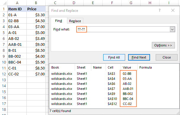
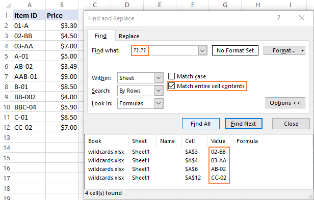
Technically, strings like AAB-01 or BB-002 also match the criteria because they do contain a ??-?? substring. To exclude these from the results, click the Options button, and check the Match entire cell contents box. Now, Excel will limit the results to only the ??-?? strings:
How to replace with wildcard
In case your data contains some fuzzy matches, wildcards can help you quickly locate and unify them.
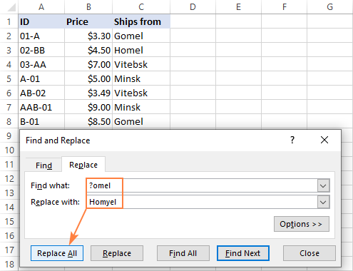
In the screenshot below, you can see two spelling variations of the same city Homel and Gomel. We'd like to replace both with another version - Homyel. (And yes, all three spellings of my native city are correct and generally accepted :)
To replace partial matches, this is what you need to do:
- Press Ctrl + H to open the Replace tab of the Find and Replace dialog.
- In the Find what box, type the wildcard expression: ?omel
- In the Replace with box, type the replacement text: Homyel
- Click the Replace All button.
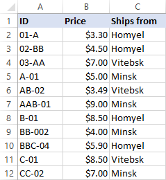
And observe the results:
How to find and replace wildcard characters
To find a character that Excel recognizes as a wildcard, i.e. a literal asterisk or question mark, include a tilde (~) in your search criteria. For example, to find all the entries containing asterisks, type ~* in the Find what box:
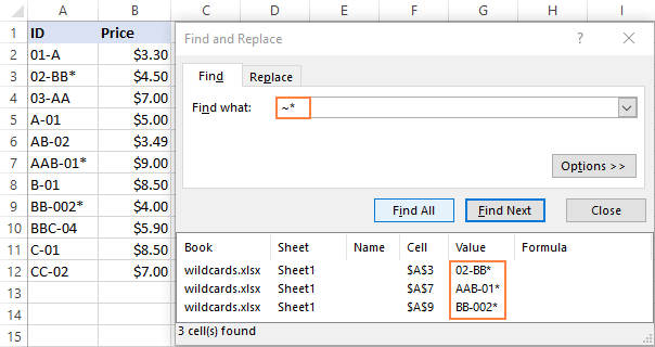
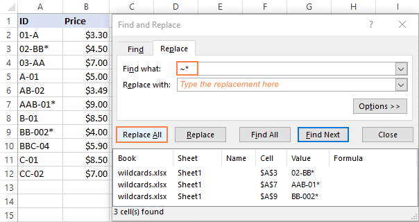
If you'd like to replace the asterisks with something else, switch to the Replace tab and type the character of interest in the Replace with box. To remove all the found asterisk characters, leave the Replace with box empty, and click Replace all.
Filter data with wildcards in Excel
Excel wildcards also come very useful when you have a huge column of data and wish to filter that data based on condition.
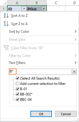
In our sample data set, supposing you want to filter the IDs beginning with "B". For this, do the following:
- Add filter to the header cells. The fastest way is to press the Ctrl + Shift + L shortcut.
- In the target column, click the filter drop-down arrow.
- In the Search box, type your criteria, B* in our case.
- Click OK.
This will instantly filter the data based on your wildcard criteria like show below:
Wildcards can also be used with Advanced Filter, which could make it a nice alternative to regular expressions (also called regexes by tech gurus) that Excel does not support. For more information, please see Excel Advanced Filter with wildcards.
Excel formulas with wildcard
First off, it should be noted that quite a limited number of Excel functions support wildcards. Here is a list of the most popular functions that do with formula examples:
AVERAGEIF with wildcards - finds the average (arithmetic mean) of the cells that meet the specified condition.
AVERAGEIFS - returns the average of the cells that meet multiple criteria. Like AVERAGEIF in the above example allows wildcards.
COUNTIF with wildcard characters - counts the number of cells based on one criterion.
COUNTIFS with wildcards - counts the number of cells based on multiple criteria.
SUMIF with wildcard- sums cells with condition.
SUMIFS - adds cells with multiple criteria. Like SUMIF in the above example accepts wildcard characters.
VLOOKUP with wildcards - performs a vertical lookup with partial match.
HLOOKUP with wildcard - does a horizontal lookup with partial match.
XLOOKUP with wildcard characters - performs a partial match lookup both in a column and a row.
MATCH formula with wildcards - finds a partial match and returns its relative position.
XMATCH with wildcards - a modern successor of the MATCH function that also supports wildcard matching.
SEARCH with wildcards - unlike the case-sensitive FIND function, case-insensitive SEARCH understands wildcard characters.
If you need to do partial matching with other functions that do not support wildcards, you will have to figure out a workaround like Excel IF wildcard formula.
The following examples demonstrate some general approaches to using wildcards in Excel formulas.
Excel COUNTIF wildcard formula
Let's say you wish to count the number of cells containing the text "AA" in the range A2:A12. There are three ways to accomplish this.
The easiest one is to include wildcard characters directly in the criteria argument:
=COUNTIF(A2:A12, "*AA*")
In practice, such "hardcoding" is not the best solution. If the criteria changes at a later point, you'll have to edit your formula every time.
Instead of typing the criteria in the formula, you can input it in some cell, say E1, and concatenate the cell reference with the wildcard characters. Your complete formula would be:
=COUNTIF(A2:A12,"*"&E1&"*")
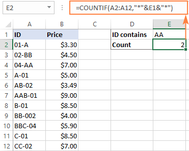
Alternatively, you can input a wildcard string (*AA* in our example) in the criteria cell (E1) and include only the cell reference in the formula:
=COUNTIF(A2:A12, E1)
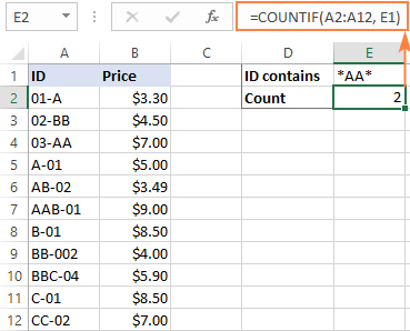
All three formulas will produce the same result, so which one to use is a matter of your personal preference.
Note. The wildcard search is not case sensitive, so the formula counts both upper case and lowercase characters like AA-01 and aa-01.
Excel wildcard VLOOKUP formula
When you need to look for a value that does not have an exact match in the source data, you can use wildcard characters to find a partial match.
In this example, we are going to look up the IDs that start with specific characters, and return their prices from column B. To have it done, enter the unique parts of the targets IDs in cells D2, D3 and D4 and use this formula to get the results:
=VLOOKUP(D2&"*", $A$2:$B$12, 2, FALSE)
The above formula goes to E1, and due to the clever use of relative and absolute cells references it copies correctly to the below cells.
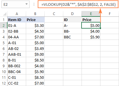
Note. As the Excel VLOOKUP function returns the first found match, you should be very careful when searching with wildcards. If your lookup value matches more than one value in the lookup range, you may get misleading results.
Excel wildcard for numbers
It is sometimes stated that wildcards in Excel only work for text values, not numbers. However, this is not exactly true. With the Find and Replace feature as well as Filter, wildcards work fine for both text and numbers.
Find and Replace with wildcard number
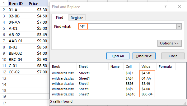
In the screenshot below, we are using *4* for the search criteria to search for the cells containing the digit 4, and Excel finds both text strings and numbers:
Filter with wildcard number
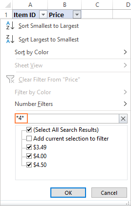
Likewise, Excel's auto-filter has no problem with filtering numbers containing "4":
Why Excel wildcard not working with numbers in formulas
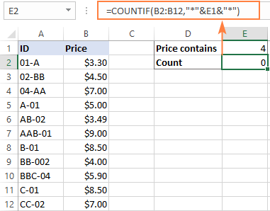
Wildcards with numbers in formulas is a different story. Using wildcard characters together with numbers (no matter whether you surround the number with wildcards or concatenate a cell reference) converts a numeric value into a text string. As the result, Excel fails to recognize a string in a range of numbers.
For instance, both of the below formulas count the number of strings containing "4" perfectly well:
=COUNTIF(A2:A12, "*4*" )
=COUNTIF(A2:A12, "*"&E1&"*" )
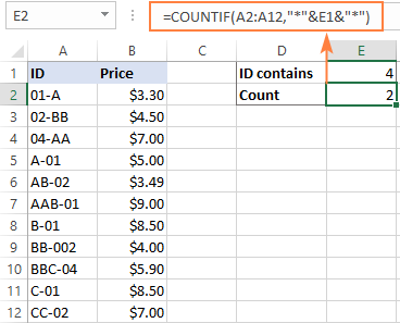
But neither can identify digit 4 within a number:
How to make wildcards work for numbers
The easiest solution is to convert numbers to text (for example, by using the Text to Columns feature) and then do a regular VLOOKUP, COUNTIF, MATCH, etc.
For instance, to get the count of cells that begin with the number in E1, the formula is:
=COUNTIF(B2:B12, E1&"*" )
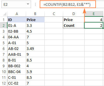
In situation when this approach is not practically acceptable, you will have to work out your own formula for each specific case. Alas, a generic solution does not exist :( Below, you will find a couple of examples.
Example 1. Excel wildcard formula for numbers
This example shows how to count numbers that contain a specific digit. In the sample table below, suppose you want to calculate how many numbers in the range B2:B12 contain "4". Here's the formula to use:
=SUMPRODUCT(--(ISNUMBER(SEARCH("4", B2:B12))))
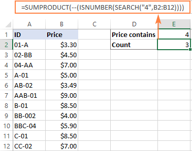
How this formula works
Working from the inside out, here's what the formula does:
The SEARCH function looks for the specified digit in every cell of the range and returns its position, a #VALUE error if not found. Its output is the following array:
{#VALUE!;1;#VALUE!;#VALUE!;3;#VALUE!;#VALUE!;1;#VALUE!;#VALUE!;#VALUE!}
The ISNUMBER function takes it from there and changes any number to TRUE and error to FALSE:
{FALSE;TRUE;FALSE;FALSE;TRUE;FALSE;FALSE;TRUE;FALSE;FALSE;FALSE}
A double unary operator (--) coerces TRUE and FALSE to 1 and 0, respectively:
{0;1;0;0;1;0;0;1;0;0;0}
Finally, the SUMPRODUCT function adds up the 1's and returns the count.
Note. When using a similar formula in your worksheets, in no case you should include "$" or any other currency symbol in the SEARCH function. Please remember that this is only a "visual" currency format applied to the cells, the underlying values are mere numbers.
Example 2. Wildcard formula for dates
The SUMPRODUCT formula discussed above works beautifully for numbers but will fail for dates. Why? Because internally Excel stores dates as serial numbers, and the formula would process those numbers, not the dates displayed in cells.
To overcome this obstacle, utilize the TEXT function to convert dates to text strings, and then feed the strings to the SEARCH function.
Depending on exactly what you aim to count, the text formats may vary.
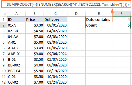
To count all the dates in C2:C12 that have "4" in the day, month or year, use "mmddyyyy":
=SUMPRODUCT(--(ISNUMBER(SEARCH("4",TEXT(C2:C12, "mmddyyyy")))))
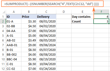
To count only the days that contain "4" ignoring months and years, use the "dd" text format:
=SUMPRODUCT(--(ISNUMBER(SEARCH("4",TEXT(C2:C12, "dd")))))
That's how to use wildcards in Excel. I hope this information will prove useful in your work. Anyway, I thank you for reading and hope to see you on our blog next week!
Practice workbook for download
Wildcards in Excel formulas (.xlsx file)
 by
by
12 comments
When using TypeScript how can you find a table name using a wildcard. For example when you create a new sheet from a Master, Excel changes the table name by adding a number. So with a name - tblHome on the Master, it becomes tblHome1 on the copied sheet.
I want to refer to any table on ActiveWorksheet with a table name "tblHome*", so it could be tblHome1 or tblHome2, or even tblHome125
We are using Excel 365 online TypeScript
Thanks
Hi! Sorry, your question is beyond the scope of the advice provided in this blog. If you have a specific question about how a function or formula works, I'll try my best to help.
Hi, thanks for the informative guide.
Seeking your advice on the following which i was unable to find similar situation and solution in the internet.
I want to filter items which cost between $240 to $260 from the below table. So only Item A & C are within the range.
Is there a formula, excel or ways to setup the information table so that i can filter easily. Thank you.
Item A: $200 to $250
Item B: $288 to $300
Item C: $250 to $300
Hi! You can filter values in Excel using either an Excel filter or FILTER formula. I recommend reading this guide: Excel Filter: How to add, use and remove.
To filter using a formula, click and read here: Excel FILTER function - dynamic filtering with formulas.
For example:
=FILTER(A1:B20,(A1:A20="A")*(B1:B20>200)*(B1:B20<250))
Thanks for your great article.
I want to find using wildcards but only replace the non wildcards part.
I.e., I have a list of mobile phone numbers starting with "44" which is the country code (e.g. 447123456789) and i want to replace the "44" with "0".
I can't just replace any "44" because there might be a "44" which is part of the actual phone number, hence I only want to replace when the "44" is at the beginning of the number.
I can use "44??????????" to 'find' them but i only want to replace the opening "44".
(PS. they all have exactly 10 digits after the 44)
Hello!
If you want to replace only the first two digits, you can use REPLACE function:
=REPLACE(A1,1,2,0)
I recommend reading this guide: How to use Find and Replace in Excel most efficiently.
Thank you, this was very helpful! I have a questions.. I am using the Find & Replace function with a wildcard and when I click replace, it does what I want and what I would expect. BUT my formatting in the cell is replaces with all CAPS and it changes the color to black.
Hi!
Find & Replace function can change the formatting of cells. Read more about it in this article: How to use Find and Replace in Excel most efficiently.
Hello,
I am seeking some assistance with how to find and replace something like this (Incident Date: 01-04-2016) where the date is always changing. Is there a wildcard string I could use after the ":" to capture all the dates? Thanks for any assistance.
mike
Hello!
You can extract a text date from your string and then convert that text to a date:
=--MID(A1,SEARCH(": ",A1)+2,20)
I hope my advice will help you solve your task.
Very interesting. Can you point me towards a discussion about ways of moving around within a formula in the formula bar? What I mean is: look for a certain symbol in the formula, then go to the beginning of the formula, then move, say, two positions to the right?
Also: is there a way of looking for wildcards and then leaving the wildcards as they are but inserting, say, brackets around them?
Finally, Excel regards -2^2 as +4, but logic suggests that it should be -4. Isn't there a macro available to retain the negativity of all minus numbers raised to even powers?
Many thanks for your help and suggestions.
Hello!
Read this guide: The order in which Excel calculations are performed. This order applies everywhere. To exponentiate a negative number, use parentheses.
(-2)^2