How to find top or bottom N values in Excel

Excel formula to find top 3, 5, 10, etc. values

To get the highest N values in a list, use the LARGE and ROWS functions together in this way:

For example, to find top N values in B2:B12, you enter the below formula in the topmost cell where you want the results to appear (D2), and then drag it through as many cells as needed.

=LARGE($B$2:$B$12, ROWS(A$2:A2))

To pull top 3 values, copy the formula to 3 cells.

To get top 5 values, copy the same formula to 5 cells.

To find top 10 values in a column, copy the formula to 10 cells.

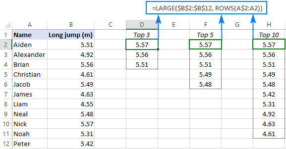
How this formula works:

The LARGE function compares all the numeric values in a range supplied for the 1^st argument (array) and returns the largest value based on the position specified in the 2^nd argument (k).

The ROWS function with an expanding range reference like ROWS(A$2:A2) generates the k values automatically. To create such a reference, we lock the row coordinate in the first cell with an absolute reference (A$2) and use a relative reference for the last cell (A2).

In the topmost cell where you enter the formula (D2 in this example), ROWS(A$2:A2) generates 1 for k, telling LARGE to return the max value. When copied to the below cells, the range reference expands by 1 row causing the k argument to increment by 1. For example, in D3, the reference changes to A$2:A3. The ROWS function counts the number of rows in A$2:A3 and returns 2 for k, so the LARGE function outputs the 2^nd largest value.

Please note that we used A$2:A2 just for convenience because our data begins in row 2. You can use any column letter and any row number for the expanding range reference, say A$1:A1 or C$1:C1.

Excel formula to get bottom 3, 5, 10, etc. values in Excel

To find the lowest N values in a list, the generic formula is:

In this case, we use the SMALL function to extract the k-th smallest value and the ROWS function with an expanding range reference to generate the k number.

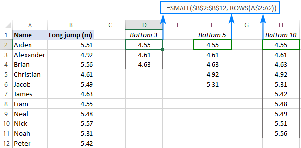
For example, to find bottom N values in the table below, use this formula:

=SMALL($B$2:$B$12, ROWS(A$2:A2))

Enter it in the topmost cell, and then drag down through as many cells as many values you want to get.

Excel formula to find top N values in a row

If your data is organized horizontally in rows, then you can use the following generic formulas to find the highest or lowest values:

Get top values in a row:

Get bottom values in a row:

The formulas' logic is the same as in the previous example with the difference that you use the COLUMNS function rather than ROWS to "feed" the k value to LARGE and SMALL.

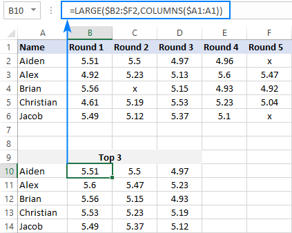
Let's say your table lists the results of 5 rounds for each participant like shown in the image below. You aim to find top 3 values in each row.

To have it done, enter the following formula in the upper-right cell (B10 in our case), and then drag it down and to the right:

=LARGE($B2:$F2, COLUMNS($A1:A1))

For the formula to copy correctly, we use a mixed reference for the array argument of LARGE that locks only the column coordinates ($B2:$F2).

To find bottom 3 values in each row, you can use an analogous SMALL formula:

=SMALL($B$2:$H$2, COLUMNS($A2:A2))

How to get matches of largest N values

In situation when you want to retrieve data relating to top values, use the classic INDEX MATCH formula together with LARGE as the lookup value:

Where:

• Return_array is a range from which to extract associated data (matches).
• Lookup_array is a range where to search for the largest values.
• K is position of the highest value to look for.

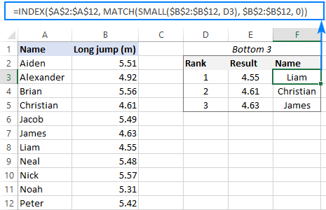
In the table below, you can find top 3 values by using the following approach.

To extract top 3 results, the formula in E3 is:

=LARGE($B$2:$B$12, D3)

Because the ranks are typed in separate cells, the ROWS function is not needed in this case - we simply reference the cell containing the k value (D3).

To retrieve the names, the formula in F3 is:

=INDEX($A$2:$A$12, MATCH(LARGE($B$2:$B$12, D3), $B$2:$B$12, 0))

Where A2:A12 are the names (return_array), B2:B12 are the results (lookup_array) and D3 is the position from largest (k).

In a similar manner, you can get matches of bottom N values. For this, just use the SMALL function instead of LARGE.

To get bottom 3 results, the formula in E3 is:

=SMALL($B$2:$B$12, D3)

To pull the names, the formula in F3 is:

=INDEX($A$2:$A$12, MATCH(SMALL($B$2:$B$12, D3), $B$2:$B$12, 0))

How this formula works:

The LARGE function gets the k-th largest value and passes it to the lookup_value argument of MATCH.

For instance, in F3, we are looking for the 1^st largest value, which is 5.57. So, after replacing the LARGE function with its output, the formula reduces to:

=INDEX($A$2:$A$12, MATCH(5.57, $B$2:$B$12, 0))

The MATCH function determines the relative position of 5.57 in B2:B12, which is 9. This number goes to the row_num argument of INDEX, simplifying the formula further:

=INDEX($A$2:$A$10, 9)

Finally, the INDEX function returns the value from the 9^th row in the range A2:A12, which is "Nick".

How to find top values with duplicates

The approach used in the previous example works fine for a dataset that has only unique numbers in the lookup column. Duplicates may lead to wrong results. For example, if the 1^st and 2^nd largest numbers happen to be the same, the LARGE function will return the same value for each, which is expected by design. But because MATCH returns the position of the first found match, the formula will output the first match twice like shown on the image below:

To "break ties" and fix the problem, we need a more sophisticated MATCH function:

=INDEX($A$2:$A$12, MATCH(1, ($B$2:$B$12=LARGE($B$2:$B$12, D2)) * (COUNTIF(F$1:F1, $A$2:$A$12)=0), 0))

In all versions except Excel 365, it only works as an array formula. So, please remember to press Ctrl + Shift + Enter to complete the formula correctly.

How this formula works:

Here, the MATCH function is configured to search for the number 1, which is the lookup value. The lookup array is constructed using the following logic:

Firstly, all the numbers are compared against the value returned by LARGE:

$B$2:$B$12=LARGE($B$2:$B$12, D2)

Secondly, the COUNTIF function with an expanding range reference checks if a given item is already in the top list. Please pay attention that the expanding range begins on the above row (F1) to avoid a circular reference.

COUNTIF(F$1:F1, $A$2:$A$12)=0

The result of the above operations are two arrays of TRUE and FALSE values, which are multiplied by each other. For example, in F3, we have the following arrays:

{FALSE;FALSE;TRUE;FALSE;FALSE;FALSE;FALSE;FALSE;TRUE;FALSE;FALSE} * {TRUE;TRUE;FALSE;TRUE;TRUE;TRUE;TRUE;TRUE;TRUE;TRUE;TRUE}

In the first array, there are two TRUE values that correspond to 5.57 (rank 1 and 2) - items 3 and 9. But in the second array, item 3 is FALSE because this name (Brian) is already in the list. The multiplication operation changes the logical values TRUE and FALSE into 1 and 0, respectively. And because multiplying by zero always gives zero, only item 9 "survives":

{0;0;0;0;0;0;0;0;1;0;0}

The MATCH function searches for "1" in this array, and returns its relative position (9), which is Nick.

How to find top values in Excel with criteria

To get top values that match certain condition, express your criteria with the help of the IF function and nest them inside the formulas discussed in the previous sections.

As an example, let's find top 3 results in a given group. To have it done, we input the target group in F1 and type the ranks 1 to 3 in E5:E7 (please see the image below).

To extract top 3 results, enter the below formula in F5 and drag it though F7:

=LARGE(IF($B$2:$B$12=$F$1, $C$2:$C$12), E5)

To ensure that the LARGE function is only processing the results within the target group, we build an IF statement that compares a list of groups against F1.

To get the names, copy this formula in G5 through G7:

=INDEX($A$2:$A$12, MATCH(LARGE(IF($B$2:$B$12=$F$1, $C$2:$C$12), E5), IF($B$2:$B$12=$F$1, $C$2:$C$12), 0))

Here, we use the already familial INDEX MATCH LARGE combination but extend it with two logical tests:

LARGE(IF($B$2:$B$12=$F$1, $C$2:$C$12), E5) - IF checks if a group matches the target one in F1. The matches get into the array from which the LARGE function picks the highest value based on the rank in E5. The result becomes the lookup value for MATCH.

IF($B$2:$B$12=$F$1, $C$2:$C$12) - IF filters out irrelevant groups again, so only the results that belong to the target group make it into the lookup array, where MATCH searches for the lookup value.

These are array formulas that should be entered by pressing Ctrl + Shift + Enter simultaneously. Due to the ability of Excel 365 to handle arrays natively, it's sufficient to press the Enter key in this version.

In Excel 365, you can perform the same logical tests inside XLOOKUP and get the identical results:

=XLOOKUP(LARGE(IF($B$2:$B$12=$F$1, $C$2:$C$12), E5), IF($B$2:$B$12=$F$1, $C$2:$C$12), $A$2:$A$12)

How to FILTER top or bottom values in Excel

In Excel 365, there is a simpler way to find largest N values by using new dynamic array functions such as SORT and FILTER.

Where:

• Data is the source table excluding column headers.
• Numbers are the numeric values to rank.
• N is the number of top entries to extract.
• Sort_index the number of the column to sort by.

For example, to filter top 3 records in our set of data, the formula goes as follows:

=SORT(FILTER(A2:B12, B2:B12>=LARGE(B2:B12, 3)), 2, -1)

In this case, we set n to 3 because we're extracting top 3 results and sort_index to 2 since the numbers are in the second column.

The beauty of this formula is that you only need to enter it in one cell, and Excel automatically spills the results into as many cells as needed (this concept is called a spill range).

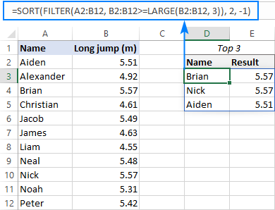
To extract the lowest 3 results, the formula is:

=SORT(FILTER(A2:B12, B2:B12<=SMALL(B2:B12, 3)), 2, 1)

How these formulas work:

Here, we use the FILTER function to filter the source data based on the criteria included in the 2^nd argument.

To get top values, we construct the logical expression that checks if a given number is greater than or equal to the Nth highest number in the list (the 3rd largest number in our case): B2:B12>=LARGE(B2:B12, 3).

To get bottom values, we check if a number is less than or equal to the 3rd lowest number: B2:B12<=SMALL(B2:B12, 3).

The result of the logical test is an array of TRUE and FALSE values, which is used for filtering - only the entries corresponding to TRUE get into the final array:

=SORT({"Aiden",5.51;"Brian",5.57;"Nick",5.57}, 2, -1)

As you can see above, the FILTER function outputs the items in the same order they appear in the source range. To sort the results, we place the FILTER formula inside the SORT function and set the sort_order argument to either -1 (descending) or 1 (ascending).

Practice workbook for download

Excel formulas to find top or bottom values (.xlsx file)