This tutorial is introducing the new Excel LET function that makes intricate formulas look more comprehensible and calculate faster.
If you work with lengthy formulas in Excel, then you are certainly familiar with the idea of named ranges that make complex formulas easier to read. And now, Microsoft is making a step further and allows assigning names to calculations and values directly in a formula. If your formula uses the same expression several times, you can let Excel calculate it just once, store the result inside a formula and reuse as many times as needed. Sounds exciting, isn't it?
Excel LET function
The Excel LET function allows you to assign names to calculation results and define variables inside a formula, so that the formula looks clearer and works faster.
Essentially, the concept is the same as naming cells, ranges and formulas in the Name Manager. What makes the LET function different is that the declared names only exist in the scope of a given formula and nowhere else.
Syntax
LET has the following syntax and arguments:
Where:
- Name1 (required) - the first name to assign. It must begin with a letter.
- Name_value1 (required) - the value or calculation assigned to name1.
- Name2 / name_value2 (optional) - the second name and value.
- Calculation (required) - a calculation that uses assigned names and values.
The function can process up to 126 name/value pairs.
Note. Microsoft uses a slightly different syntax notation:
LET(name1, name_value1, calculation_or_name2, [name_value2, calculation_or_name3…])
I personally find it a little confusing, so I put it in a more customary form. Basically, they talk about the same thing but in different ways.
Availability
The LET function is only available in these versions of Excel:
- Excel 365 (for Windows and Mac)
- Excel 2021 (for Windows and Mac)
- Excel for the web
Basic LET formula
If you do not have a clear understanding of the function yet, an example of the LET formula in its simplest form will help bring the essentials into focus.
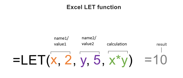
Consider this simple expression: x+y. Here, we have 2 variables, x and y. Let's assign the value 2 to x, the value 5 to y and multiply one by the other:
=LET(x, 2, y, 5, x*y)
Enter this formula in a cell, and it will return 10 as the result.
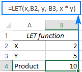
Instead of values, the variables can be assigned to cell references, say x to B2 and y to B3:
=LET(x,B2, y, B3, x * y)
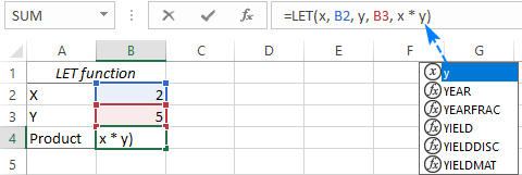
To ease building a formula, the already declared names appear in the intellisense drop down list, just like the names defined in the name manager.
Looking at the above formula you may be wondering, what's the point in over-complicating things? Why not simply put:
=B2*B3
In this particular case, a normal multiplication is of course simpler. The purpose is to clarify the concept. When it comes to more complex formulas with repeated calculations, the LET function takes on a whole new degree of usefulness as demonstrated in the further examples.
Advantages
If you still doubt that LET will be a worthy addition to your Excel toolbox, then consider these benefits:
Simplified formulas. Giving descriptive names to variables and intermediate calculations makes it easier to understand what the formula is actually doing. You no longer need to figure out the inner logic of each specific expression or reference in a formula.
Faster calculations. When the same expression is repeated in a formula multiple times, Excel calculates it multiple times. When the expression is referred by name, Excel calculates it only once. As the result, a whole worksheet recalculates much faster. This positive effect on performance is especially noticeable in case of long formulas and huge data sets.
Easy maintenance. Using names for repeated calculations not only makes formulas more compact but also easier to update. When adjustments are needed, you make just a single change instead of updating the same expressions multiple times, thus saving time and reducing a change of human errors.
Usage notes
To shorten the learning curve and prevent common errors, please follow these simple guidelines:
- A LET formula should have an odd number of arguments - one or several name/value pairs and a calculation. The last argument must always be a calculation that returns the final result.
- When assigning names in your LET formulas, ensure they comply with Excel's naming conventions. This means names should not include spaces or punctuation marks, must not conflict with cell references, etc.
- For clarity, avoid using names that are already used in the Name Manager. If the same name is assigned inside LET and defined in the name manager, the name manager version will be ignored.
- The names declared within a LET formula are only applicable within the scope of that formula itself.
How to use LET function in Excel - formula examples
And now, it's time to look at more realistic use cases and reveal the whole power of the new function.
Example 1. LET formula to reduce repeated calculations
When writing multi-level formulas, it often happens that the same expression or calculation is used more than once. A typical example is nested IF statements. In this context, let's see how LET can simplify things.
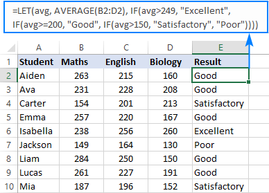
Supposing you have the results of student exams in three different subjects (columns B, C and D). You want to find an average for each student and grade it as shown in the table on the right:
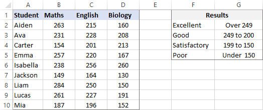
The AVERAGE function can easily compute an arithmetic mean for each row:
AVERAGE(B2:D2)
And then, you build a nested IF statement based on the above criteria.
=IF(AVERAGE(B2:D2)>249, "Excellent", IF(AVERAGE(B2:D2)>=200, "Good", IF(AVERAGE(B2:D2)>150, "Satisfactory", "Poor")))
The problem is the same AVERAGE function is repeated three times. Well, maybe not really a problem, but an unnecessary complication that forces Excel to perform the same calculation thrice.
To optimize the formula, we can assign a name to the AVERAGE function (say, avg) and replace the function with this "local" name. This way, an average is calculated just once helping the formula run faster:
=LET(avg, AVERAGE(B2:D2), IF(avg>249, "Excellent", IF(avg>=200, "Good", IF(avg>150, "Satisfactory", "Poor"))))
Enter the formula in E2, drag it down through E10, and you'll get this result:
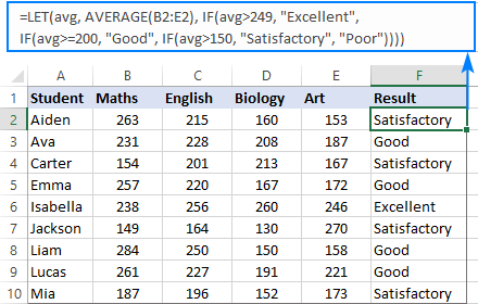
Imagine you add one more exam (column E) to the source table. Naturally, you wish to include that in the average. Without LET, you'd have to perform this adjustment in the logical test of every IF function. Being a human being, you might overlook something and fail to update all the references correctly. With LET, you make just a single change:
=LET(avg, AVERAGE(B2:E2), IF(avg>249, "Excellent", IF(avg>=200, "Good", IF(avg>150, "Satisfactory", "Poor"))))
Example 2. LET with multiple names
Here's another example showing how the LET function can ease the creation of complex formulas.
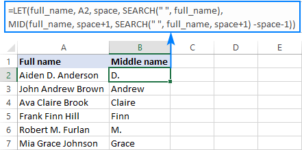
Let's say you have a list of full names (column A) from which you wish to extract middle names. The below formula does the job perfectly, but at first sight its logic is quite obscure:
=MID(A2, SEARCH(" ", A2) + 1, SEARCH(" ", A2, SEARCH(" ", A2) +1) - SEARCH(" ", A2) - 1)
To provide some meaningful context to yourself and other users, you can define a couple of names such as:
- full_name - A2
- space - SEARCH(" ", full_name)
Obviously, cell A2 contains a full name that needs to be split, and the SEARCH function returns the position of the first space character in the name.
And then, we replace the cell reference and the SEARCH function with the declared names.
=LET(full_name, A2, space, SEARCH(" ", full_name), MID(full_name, space + 1, SEARCH(" ", full_name, space + 1) - space - 1))
If you are familiar with the MID syntax, the formula becomes much easier to comprehend:
To the position of the first space, you add 1 to start the extraction from the next character (space+1). To get the length of the middle name (i.e. how many characters to extract from the full name), you determine the position of the second space by nesting one SEARCH function into another, then find the difference between the positions of the two spaces and subtract 1 from the result to eliminate a trailing space (SEARCH(" ", full_name, space+1) - space -1)).
For better readability, you can wrap the names and calculation onto separate lines like this:
Example 3. LET function with dynamic arrays
In the previous examples, the LET function operated on a single cell, and we copied the formula to the below cells. However, LET can also accept arrays as input and produce arrays as output. This is possible due to Excel 365's new calculation engine and dynamic arrays.
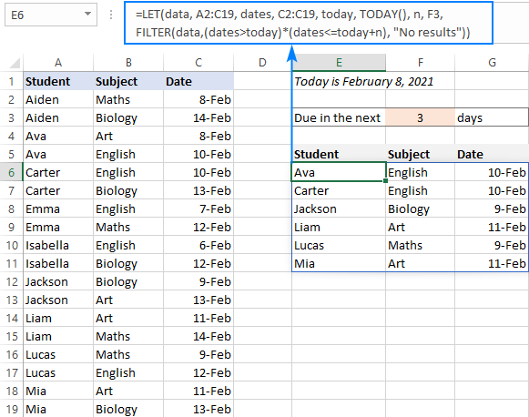
From the below table, suppose you want to get a list of exams that are to be taken in the next n days, not including today. This can be done by using the FILTER function with multiple criteria:
FILTER(data, (dates>today) * (dates<=today+n), "No results")
All you need to do is to define the corresponding names:
- data - A2:C19
- dates - C2:C19
- today - TODAY()
- n - F3
After that, put the names and FILTER formula inside LET:
=LET(data, A2:C19, dates, C2:C19, today, TODAY(), n, F3, FILTER(data, (dates>today) * (dates<=today+n), "No results"))
The result is an array of records matching the specified criteria:
Excel LET function not working
If you cannot find the LET function in your Excel or your formula results in error, that may happen because of the following reasons:
There is no LET function in my Excel
The LET function is only available in these Excel versions. The function is not backward compatible and won't appear in earlier Excel versions.
#NAME? error
As there's a very slim chance that someone may misprint the function's name, the problem is most likely with assigned names. Please make sure you've declared each name used in the calculation and all of the names are spelled correctly.
Invalid names
If you encounter a "there's a problem with this formula" error message while inputting a LET formula, it could be due to improperly defined names. For instance, names like "Abc1" or "Fun1" won't be accepted since they coincide with cell references ABC1 or FUN1. This clash leads to internal conflicts, causing Excel to display an error. To avoid such errors, ensure that names are unique and compliant with Excel naming rules.
That's how you can simplify and speed up your calculations with the help of the LET function. I thank you for reading and hope to see you on our blog next week!
Practice workbook for download
Excel LET formula examples (.xlsx file)
 by
by
16 comments
Could someone please comment why seq is not a range? Ultimately, I like to mark blocks of trues & falses with sequential numbers that incrementally goes from 1 to n. There are more calculation beyond this but I just like to get pass this hump 1st. Thank you.
=LET(
range, A2:A10,
med, MEDIAN(range),
tf, range > med,
seq, IF(ROW(A2:A10)=ROW(A2), 1, IF(tfOFFSET(tf,-1,0), OFFSET(seq,-1,0)+1, OFFSET(seq,-1,0))),
seq
)
Hello Kyle!
The provided Excel formula generates a sequence of numbers that increases whenever a block of "TRUE" values is encountered in the tf array. However, this formula has some issues:
tfOFFSET(tf,-1,0): This part of the formula seems to be incorrect. The OFFSET function requires a valid reference as its first argument. Using tfOFFSET directly is likely to cause an error.
OFFSET(seq,-1,0): This part of the formula also has a potential issue. If you’re not careful with how you define or initialize your sequence, using OFFSET(seq,-1,0) can cause some unexpected results or errors.
Please try the following formula:
=LET(
range, A2:A10,
med, MEDIAN(range),
tf, range > med,
seq, SCAN(0, tf, LAMBDA(a, b, IF(b, a+1, 1))),
seq
)
LET function helps define and reuse intermediate values in formulas, making them more readable and maintainable.
range, A2:A10: This defines the range of cells containing the data.
med, MEDIAN(range): This calculates the median of the data in the range.
tf, range > med: This creates an array of TRUE/FALSE values based on whether each value in the range is greater than the median.
seq, SCAN(0, tf, LAMBDA(a, b, IF(b, a+1, 1))): This is the core of the formula.
SCAN is a powerful function that iterates through an array and accumulates a result.
0 is the initial value of the sequence.
tf is the array of TRUE/FALSE values.
LAMBDA(a, b, IF(b, a+1, 1)) is the lambda function that defines how the sequence is updated:
If the current value of tf is TRUE (b is TRUE), the previous value of the sequence (a) is incremented by 1.
If the current value of tf is FALSE (b is FALSE), the sequence is reset to 1.
We have a special tutorial on LAMBDA function. Please see: Excel LAMBDA function: how to write and use.
This formula assigns sequential numbers to blocks of TRUE values.
Alexander, thank you for responding. I have something like this, which is different from your above.
=LET(range, M3:M10000, med, MEDIAN(range), tf, range<med, seq, SCAN(0, tf, LAMBDA(a,b, IF(a = 0, 1, IF(INDEX(tf, ROW(tf) - 1) b, a + 1, a)))), seq)
The idea here is to prime the 1st entry of seq with 1, hence the if(a=0,1 then all subsequent evaluation will hinge upon the change in tf as it traverses down the list. If there's a change we take the prior value of a, which will be 1 & increment to 2. If there's no change it'll be the prior value. So, in seq, I'll eventually get blocks of 1s, 2s, 3s, etc. rather than trues/falses. With this I was hoping to build a histogram with unique_seq, unique(seq). Unfortunately, even my version of the seq is not working. Excel gives me #CALC!. There must be some sort of recursion going on there that I can't see.
Hi! I wrote this formula based on the description you provided in your original comment. Please note that if you’d provided me with the precise and detailed description of your task from the very beginning, I’d have created a different formula that would have worked for your case.
To understand what you want to do, give an example of the source data and the expected result.
Alexander, apologies. My initial task is to take a timeseries, assess its median/average or whatever. Compute blocks of true/false based on above or below its median. But I can't build a meaningful histogram with true/false blocks. So, I'll need to label each block starting with 1 & incrementally increasing for other blocks. Say, I have 1st block of trues then this will be 1s, next block of falses will be 2s, next true will be 3s, etc. Once, I have all these blocks of numbers I can get unique of the sequence (seq), call that unique_seq. Then I could build a histogram based on the count of each occurrence. This will yield an array of integer numbers. Finally, I can assess its average. This will give me the average days that the time series will flip back and forth betwixt its median/average or whatnot. I hope this helps. Thanks in advance.
Hi! Unfortunately, your description did not help to understand the problem. I can't guess what it means: "1st block of trues then this will be 1s, next block of falses will be 2s, next true will be 3s", "get unique of the sequence". I asked for an example of source data and desired result.
Alexander, thank you for your patience. The Series is Column AV, TF is AW, Seq is AX, Unique is AY, Histogram is AZ. The data for AV starts at row 3. TF is =AV3>AV$2, where AV$2 is some arbitrary number 16. So, 1st 3 rows are TRUE, then followed by 1 FALSE, then 13 TRUE, etc. Seq is =IF(AW3AW2,AX2+1,AX2). If the current row is different from the previous then add 1 to the previous value of Seq; otherwise, it's the previous value of Seq. Unique is just =UNIQUE(AX3:AX135), the unique of the entire Seq. Finally, Histogram is =COUNTIF(AX3:AX134,AY3). It's counting the occurrences of each Unique element amongst the entire Seq. So, for the 1st 3 rows of Histogram I have 3,1,13, etc. With this I can then do average/median or whatnot. Using the LET function fails when assessing Seq using scan & lambda combo for whatever reason. It would be nice to get over this hurdle. Thank you.
Series TF Seq Unique Histogram
16
17.19 TRUE 1 1 3
16.62 TRUE 1 2 1
16.55 TRUE 1 3 13
15.77 FALSE 2 4 4
17.05 TRUE 3 5 4
18.13 TRUE 3 6 4
19.77 TRUE 3 7 1
18.57 TRUE 3 8 9
18.14 TRUE 3 9 1
18.86 TRUE 3 10 4
18.47 TRUE 3 11 1
19.96 TRUE 3 12 1
19.33 TRUE 3 13 1
18.93 TRUE 3 14 8
18.67 TRUE 3 15 1
18.49 TRUE 3 16 1
18.08 TRUE 3 17 4
15.96 FALSE 4 18 3
15.97 FALSE 4 19 13
15.28 FALSE 4 20 38
15.5 FALSE 4 21 1
16.3 TRUE 5 22 6
16.08 TRUE 5 23 2
17.03 TRUE 5 24 2
16.78 TRUE 5 25 3
15.39 FALSE 6 26 4
Hi! I'm really sorry, we cannot help you with this task. Solving this complex problem requires more than a single formula.
I'm trying to paste my snippet of the Excel but all the coloring is gone. I'll explain it here. 1st 2 rows are just "headers." 16 is just a number I chose. I could be median/average of the Timeseries below. The TF column has True/False, true if series>16, false if not. Seq has 1s, 2s, 3s, etc. It's enumeration of each block of true/false. The formula is "=IF(BA3BA2,BB2+1,BB2)" This is what the formula is doing: if(TF[current]TF[Prev],Seq[Prev]+1,Seq[Prev]). The Unique column is just unique(Seq3:Seq1000). Histogram is countif(Seq,Histogram) "=COUNTIF(BB:BB,BC3)" Finally, 2 is median(Histogram) & 14.169 is average(Histogram).
I was trying to encode all this in a LET(). But I think the sequencing using lambda() wasn't working at all. It's probably not lambda but usage of referencing currentprev logic using index or offset that Excel/Google Sheets do not understand well. I hope this helps.
16 TF Seq Unique Histogram 2 Median Days TF Flips
Timeseries 14.16901408 Average Days TF Flips
17.19 TRUE 1 1 3
16.62 TRUE 1 2 1
16.55 TRUE 1 3 13
15.77 FALSE 2 4 4
17.05 TRUE 3 5 4
18.13 TRUE 3 6 4
19.77 TRUE 3 7 1
18.57 TRUE 3 8 9
18.14 TRUE 3 9 1
18.86 TRUE 3 10 4
18.47 TRUE 3 11 1
19.96 TRUE 3 12 1
19.33 TRUE 3 13 1
18.93 TRUE 3 14 8
18.67 TRUE 3 15 1
18.49 TRUE 3 16 1
18.08 TRUE 3 17 4
15.96 FALSE 4 18 3
15.97 FALSE 4 19 13
15.28 FALSE 4 20 38
15.5 FALSE 4 21 1
16.3 TRUE 5 22 6
16.08 TRUE 5 23 2
17.03 TRUE 5 24 2
16.78 TRUE 5 25 3
Hi! Unfortunately, your explanations for the 4th and 5th columns are not quite clear, the formula is not fully written down. It is very difficult to understand what data the formula “=COUNTIF(BB:BB,BC3)” uses. Perhaps it is referring to itself.
Oz,
Thank you for the post. The concept of joining multiple arrays or ranges would be very powerful and a concept that I have researched previously and continue to monitor for in Excel. However, I have yet to find a functional example of this. I attempted to run your example function and after correcting for quotes in the function received the following results:
"A year consists of 1 months. Of which, only 1 hot months, where the hottest among them are: Jun, Jul, Aug. allM is an error = TRUE"
Anything I attempt to run on coldM, hotM, or allM results in #VALUE for the function indicating that the array is an error as noted above and in the formula below.
Here is my formula:
=LET(
autumnM, {"Sep","Nov","Oct"},
winterM, {"Dec","Jan","Feb"},
springM, {"Mar","Apr","May"},
summerM, {"Jun","Jul","Aug"},
coldM, autumnM:winterM,
hotM, springM:summerM,
allM, coldM:hotM,
CONCATENATE("A year consists of ", COUNTA(allM), " months. Of which, only ", COUNTA(hotM), " hot months, where the hottest among them are: ", TEXTJOIN(", ", TRUE, summerM), ". allM is an error = ", ISERROR(allM)))
Hello!
You cannot concatenate arrays the way you are trying to do so. Here is an example of concatenating two arrays -
=LET(
b, {"Sep";"Nov";"Oct"},
a, {"Jun";"Jul";"Aug"},
s, SEQUENCE(ROWS(a) + ROWS(b)),
IF(s > ROWS(a),
INDEX(b, s - ROWS(a)),
INDEX(a, s)
))
Another interesting thing to update and mention is that, once a name was defined with its value (any type of value), each of the following names-values pairs we assign, can immediately start relating to and using it, as you can witness yourself in the parallel "LET function" article of Microsoft's ("Example 2" at the end):
https://support.microsoft.com/en-us/office/let-function-34842dd8-b92b-4d3f-b325-b8b8f9908999
So, names can be nested, to give shorter and simpler access to any granular part of them!
--------------------
For example, months of the year (by Northern Hemisphere perspective):
=LET(
autumnM , {Sep, Nov, Oct},
winterM, {Dec, Jan, Feb},
springM, {Mar, Apr, May},
summerM, {Jun, Jul, Aug},
coldM, autumnM:winterM,
hotM, springM:summerM,
allM, coldM:hotM,
CONCATENATE("A year consists of ", COUNTA(allM), " months. Of which, only ", COUNTA(hotM), " hot months, where the hottest among them are: ", TEXTJOIN(", ", TRUE, summerM), "."))
(Result: "A year consists of 12 months. Of which, only 6 hot months, where the hottest among them are: Jun, Jul, Aug.")
I want to list, in a single column, just the unique names of individuals that appear in an array 4 columns wide by any number of rows deep. I'm thinking if I built a LET formula that allows iteration through the array one cell at a time, place it in a LAMBDA, and wrap it all in UNIQUE, I can make this happen. Can't quite figure out how to build the LET function to achieve this. Can you point me in the right direction?
Excellent explanation! I came across this while searching for more info on using LET after seeing it used in a formula to reverse comma separated strings in a cell. It works well, but I was having a hard time figuring out all the various pieces. This helped tremendously in understanding how it's supposed to work and some of the ways it can be leveraged.
I've got several spreadsheets with tons of complex formulas that really tax my system (and patience) that I'll be looking at to see where I can simplify and hopefully speed up calculations.
How to fix a cell if you get "value" after creating a formula eg 3*5="value"