Learn formulas and formula-free ways to trim whitespaces, remove special symbols (even the first/last N characters) and the same text strings before/after certain chars from multiple cells at once.
Removing the same part of the text from several cells at once can be as important and tricky as adding it. Even if you know some of the ways, you will definitely find new ones in today's blog post. I share plenty of functions and their ready-made formulas and, as always, I save the easiest — formula-free — for last 😉
How to remove spaces and whitespaces in Google Sheets
Whitespace can easily slip into cells after the import or if multiple users edit the sheet at the same time. In fact, extra spaces are so common that Google Sheets has several options to solve this problem.
Built-in trim removal tool
To remove all whitespaces you can use a special built-in Google Sheets Trim tool.
Just select all Google Sheets cells where you want to remove whitespace and choose Data > Data cleanup > Trim whitespace in the spreadsheet menu:
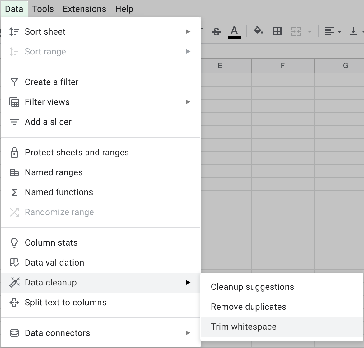
As you click the option, all leading and trailing spaces in the selection will be taken away completely while all extra spaces in-between the data will be reduced to one:
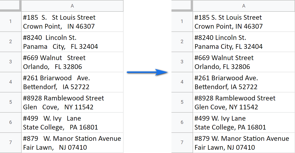
Trim function to remove spaces in Google Sheets
The menu option permanently edits your original cells to remove extra spaces one time. If you need to have a clean copy that updates automatically in another column, you can use the TRIM() formula. The function removes all spaces from a text string except for single spaces between words.
The formula is quite simple:
=TRIM(A1)
Tip: You can also use the =CLEAN() function to remove non-printing characters that TRIM() doesn't catch.
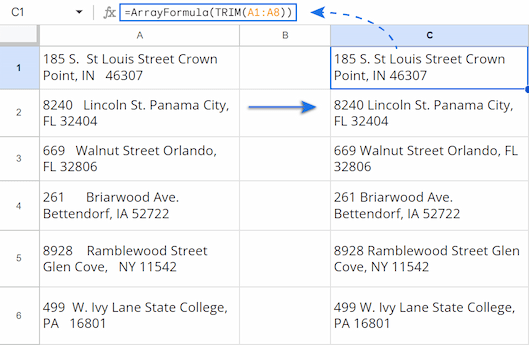
To apply a formula to the column, click and drag the plus sign down the column or wrap it in ARRAYFORMULA:
=ArrayFormula(TRIM(A1:A8))
Remove Spaces with Power Tools
If you find the menu option too basic and formulas too complex, the Power Tools add-on is the fastest and most powerful solution.
To remove spaces with Power Tools just select the range of cells you need to clean and check the box Remove spaces between words to one.
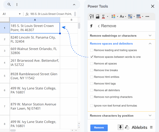
Click the Remove button, and your selected cells are cleaned in place almost instantly. Moreover, you can remove not only spaces but also line breaks, HTML entities & tags, and other delimiters and non-printing characters. Just tick off all the needed checkboxes and press Remove.
Using Power Tools is the perfect combination of the menu tool's simplicity and the formula's power without needing a separate column.
Remove other special characters from text strings in Google Sheets
Alas, Google Sheets doesn't offer a tool to 'trim' other characters but spaces. You have to deal with formulas or add-ons here.
SUBSTITUTE formula to remove characters from a string
Here I have addresses with hashtags before the apartment numbers and phone numbers with dashes and brackets in-between:

I will use formulas to remove those special characters.
The SUBSTITUTE function will help me with that. It is normally used to replace one character with another, but you can turn that to your advantage and replace the unwanted characters with… well, nothing :) In other words, remove it.
Let's see what argument the function requires:
- text_to_search is either the text to process or a cell that contains that text. Required.
- search_for is that character that you want to find and delete. Required.
- replace_with — a character you will insert instead of the unwanted symbol. Required.
- occurrence_number — if there are several instances of the character you're looking for, here you can specify which one to replace. It's completely optional, and if you omit this argument, all instances will be replaced with something new (replace_with).
So let's play. I need to find a hashtag (#) in A1 and replace it with 'nothing' which is marked in spreadsheets with double quotes (""). With all that in mind, I can build the following formula:
=SUBSTITUTE(A1,"#","")
Tip: The hashtag is also in double quotes since this is the way you should mention text strings in Google Sheets formulas.
Then copy this formula down the column if Google Sheets doesn't offer to do that automatically, and you'll get your addresses without the hashtags:

But what about those dashes and brackets? Should you create additional formulas? Not at all! If you nest multiple SUBSTITUTE functions in one Google Sheets formula, you will remove all these characters from each cell:
=SUBSTITUTE(SUBSTITUTE(SUBSTITUTE(SUBSTITUTE(A1,"#",""),"(",""),")",""),"-","")
This formula removes characters one by one and each SUBSTITUTE, starting from the middle, becomes the range to look at for the next SUBSTITUTE:
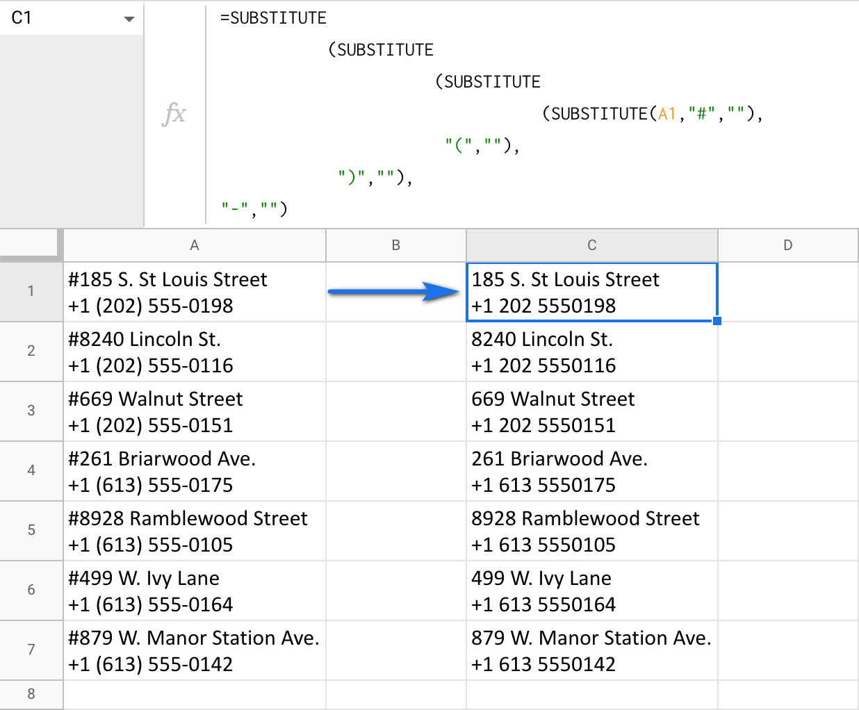
Tip: What's more, you can wrap this in ArrayFormula and cover the entire column at once. In this case, change the cell reference (A1) to your data in column (A1:A7) as well:
=ArrayFormula(SUBSTITUTE(SUBSTITUTE(SUBSTITUTE(SUBSTITUTE(A1:A7,"#",""),"(",""),")",""),"-",""))
Remove special characters with Power Tools
As you can see, the SUBSTITUTE formula works, but it gets very long and complicated if you need to remove more than one or two characters. You have to nest a new function for every single character you want to remove.
A much simpler and faster way to remove characters from a string is to use the Power Tools add-on. It lets you remove multiple substrings or individual characters from any position in all selected cells at a time.
Just select the range, type all the characters you want to remove and click Remove:
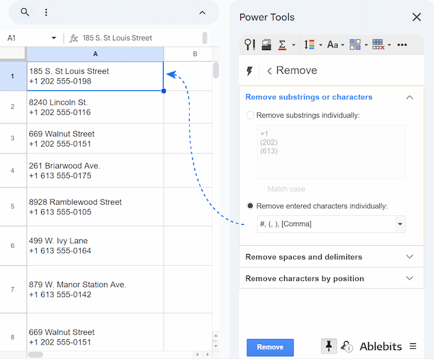
All the characters you’ve specified will be cleaned without you having to write a single formula.
Remove specific text from cells in Google Sheets
Although you can use the aforementioned SUBSTITUTE function for Google Sheets to remove text from cells, I'd like to show another function as well — REGEXREPLACE.
Google Sheets formula to remove text: REGEXREPLACE
The REGEXREPLACE function's name is an acronym from 'regular expression replace'. And I'm going to use the regular expressions to search for the strings to remove and replace them with 'nothing' ("").
Tip: If you're not interested in using regular expressions, I describe a much easier way.
Tip: If you're looking for ways to find and remove duplicates in Google Sheets, visit this blog post instead.
As you can see, there are three arguments to the function:
- text — is where you're looking for the text string to remove. It can be the text itself in double quotes or a reference to a cell/range with text.
- regular_expression — your search pattern that consists of various character combinations. You'll be looking for all strings that match this pattern. This argument is where all the fun happens, if I may say so.
- replacement — a new desired text string.
Let's suppose my cells with data also contain the country name (US) if different places in cells:

How will REGEXREPLACE help me remove it?
=REGEXREPLACE(A1,"(.*)US(.*)","$1 $2")

Here's how the formula works exactly:
- it scans the contents of the cell A1
- for matches to this mask: "(.*)US(.*)"
This mask tells the function to look for the US no matter what number of other characters may precede (.*) or follow (.*) the name of the country.
And the entire mask is put in double quotes per the function demands 🙂.
- the last argument — "$1 $2" — is what I want to get instead. $1 and $2 each represent one of those 2 groups of characters — (.*) — from the previous argument. You should mention those groups in the third argument this way so the formula could return everything that possibly stands before and after the US
As for the US itself, I simply don't mention it in the 3rd argument — meaning, I want to return everything from A1 without the US.
Tip: There's a special page you can reference to build various regular expressions and look for the text in different positions of cells.
Tip: As for those remaining commas, the SUBSTITUTE function described above will help to get rid of them ;) You can even enclose REGEXREPLACE with the SUBSTITUTE and solve everything with one formula:
=SUBSTITUTE(REGEXREPLACE(A1,"(.*)US(.*)","$1 $2"),",","")
How to remove text from a string in Google Sheets without formulas
If you're not interested in using regular expressions, a much easier way is to use Power Tools.
To remove text with Power Tools, just select the range, enter the combination of characters or words you want to delete and click Remove.
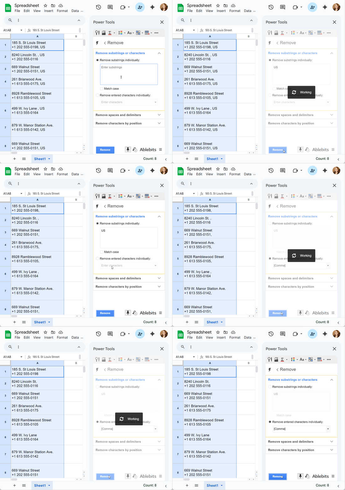
That’s it! No need for any complex formulas.
How to remove multiple substrings at once
But sometimes you need to remove several substrings simultaneously. Instead of a highly nested formula, the Power Tools add-on lets you enter a list of all the substrings you want to remove and do it in just a few clicks.
To remove multiple substrings at the same time, just type all the words you want to delete and click Remove.
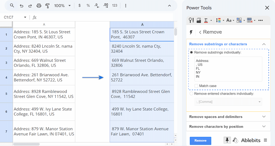
The add-on will process your entire selection, removing every instance of every word from your list.
Remove text before/after certain characters in all selected cells
Example 1. REGEXREPLACE function for Google Sheets
When it comes to getting rid of everything before and after certain characters, REGEXREPLACE also helps. Remember, the function requires 3 arguments:
And, as I mentioned above when I introduced the function, it's the second one you should use correctly so the function knows what to find and remove.
So how do I remove the addresses and keep only phone numbers in cells?

Here's the formula I will use:
=REGEXREPLACE(A1,".*\n.*(\+.*)","$1")
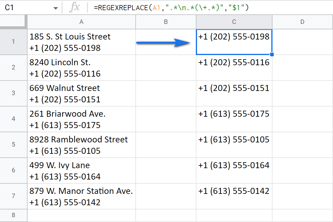
Here's the regular expression I use in this case:
- ".*\n.*(\+.*)"
- In the first part — .*\n.* — I use backslash+n to tell that my cell has more than one row. So I want the function to remove everything before and after that line break (including it).
- The second part that is in brackets (\+.*) says that I want to keep the plus sign and everything that follows it intact. I take this part in brackets to group it and keep it in mind for later.
Tip: The backslash is used before the plus to turn it into a character you're looking for. Without it, the plus would be just a part of the expression that stands for some other characters (as an asterisk does, for example).
- As for the last argument — $1 — it makes the function return that only group from the second argument: the plus sign and everything that follows (\+.*).
Tip: As an alternative, you can simply remove the first line if that'd be easier for your task:
=REGEXREPLACE(A1, "^.*", "")

In a similar fashion, you can delete all phone numbers yet keep the addresses:
=REGEXREPLACE(A1,"(.*\n).*","$1")
Only this time, you tell the function to group (and return) everything before the line break and clear out the rest:

Another case I'd like to mention here concerns the extra info in brackets. Whenever it's irrelevant, there's no point in keeping it in cells. And you have all the means to remove not just everything in-between but also the brackets themselves.
REGEXREPLACE will do that in one go:
=REGEXREPLACE(A1,"\((.*)\)","")

The formula takes:
- the symbol of the opening bracket: \(
- the symbol of the closing one: \)
- and a group of characters between them: (.*)
and replaces them with "nothing" (meaning. removes them): ""
Everything outside them stays intact.
Example 2. RIGHT+LEN+FIND
There are a few more Google Sheets functions that let you remove the text before a certain character. They are RIGHT, LEN and FIND.
Note. These functions will help only if the records to keep are of the same length, like phone numbers in my case. If they're not, just use the REGEXREPLACE instead or, even better, the Power Tools add-on
Using this trio in a particular order will help me get the same result and remove the entire text before a character — a plus sign:
=RIGHT(A1,(LEN(A1)-(FIND("+",A1)-1)))

Let me explain how this formula works:
- FIND("+",A1)-1 locates the position number of the plus sign in A1 (24) and subtracts 1 so the total doesn't include the plus itself: 23.
- LEN(A1)-(FIND("+",A1)-1) checks the total number of characters in A1 (40) and subtracts 23 (counted by FIND) from it: 17.
- And then RIGHT returns 17 characters from the end (right) of A1.
Unfortunately, this way won't help much to remove the text after the line break in my case (clear phone numbers and keep addresses), because the addresses are of different length.
Example 3. Remove characters before/after text with Power Tools
As you've seen, REGEXREPLACE does not have a very intuitive syntax and requires practice to work with, and the RIGHT+LEN+FIND method isn't flexible enough for data of different lengths. This is where the Power Tools add-on provides a much simpler solution, as it has a tool for this exact task.
To remove characters before or after text with Power Tools, you’ll need to pick the range, enter the string before/after which you'd like to remove all text and click Remove.
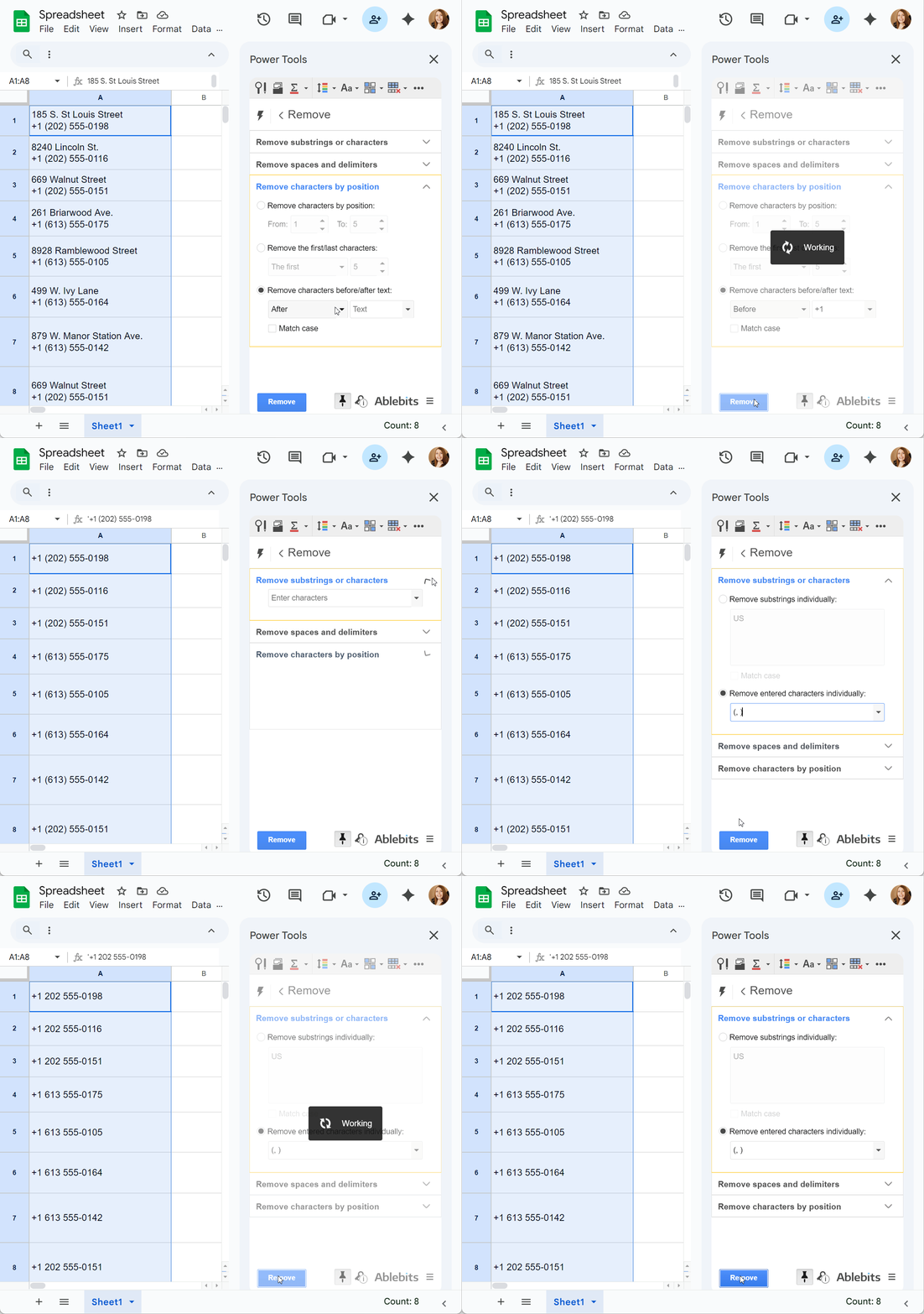
Easy-peasy and without any formulas! 😊
Remove the first/last N characters from strings in Google Sheets
Whenever you need to remove a certain number of different characters from the beginning or the end of a cell, REGEXREPLACE and RIGHT/LEFT+LEN will also help.
Note. Since I already introduced these functions above, I will keep this point short and provide some ready-made formulas.
So, how can I erase the codes from these phone numbers? Or, in other words, remove the first 9 characters from cells:

- Use REGEXREPLACE. Create a regular expression that will find and delete everything up to the 9th character (including that 9th character):
=REGEXREPLACE(A1,"(.{9})(.*)","$2")
Tip: To remove the last N characters, just swap the groups in the regular expression:
=REGEXREPLACE(A1,"(.*)(.{9})","$1") - RIGHT/LEFT+LEN also count the number of characters to delete and return the remaining part from the end or the beginning of a cell respectively:
=RIGHT(A1,LEN(A1)-9)
Tip: To remove the last 9 characters from cells, replace RIGHT with LEFT:
=LEFT(A1,LEN(A1)-9) - Last but not least is the REPLACE function. You tell it to take the 9 characters starting from the left and replace them with nothing (""):
=REPLACE(A1,1,9,"")
Note. Since REPLACE requires a starting position to process the text, it won't do if you need to delete N characters from the end of a cell.
As you can see, the formula method requires you to understand the syntax of the functions. To remove any numbers or characters easily without formulas, use the Power tools add-on.
To remove the first/last characters with Power Tools, select the range, enter the number of characters you'd like to delete, and click Remove:
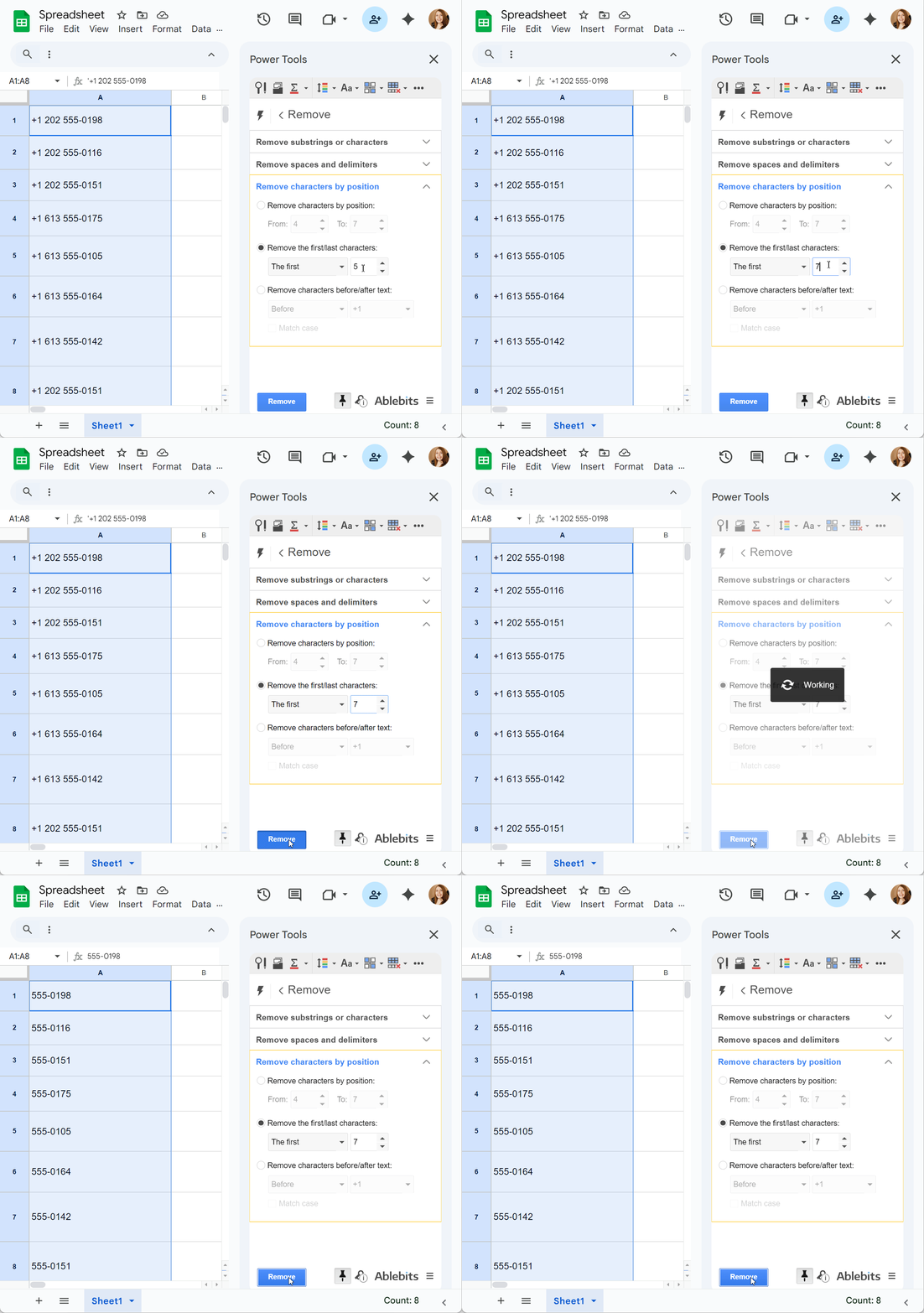
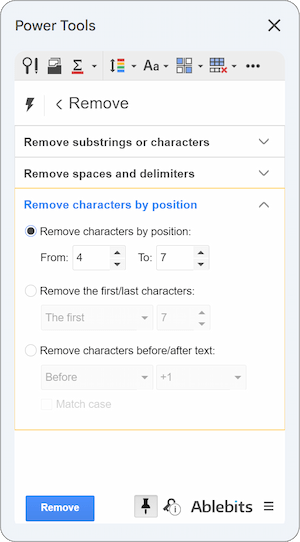
There are settings to remove text in Google Sheets by a certain position, first/last N characters, or before/after chars:
Another tool from Power Tools will remove time and date units from timestamps. It's called Split Date & Time:
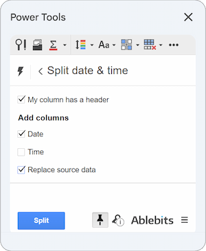
What's the splitting tool got to do with removing time and date units? Well, to remove time from timestamps, select Date since it's a part you want to keep and also tick off Replace source data, just like on the screenshot above.
The tool will extract the date unit and replace the entire timestamp with it. Or, in other words, this add-on for Google Sheets will remove the time unit from the timestamp:

So, while you can use complex formulas like SUBSTITUTE and REGEXREPLACE to clean text in Google Sheets, the easiest and most efficient way to remove spaces, special characters, or specific text in the strings is with Power Tools.
You will have all these and 40+ other time-savers for spreadsheets by installing Power Tools from the Google Store. You don't have to take my word for it, just install Power Tools in your Google Sheets and see for yourself. The first 30 days are completely free and fully functional, so you'll have the time to decide if it's worth any investment.
If you have any questions related to any part of this blog post, I'll see you in the comments section below!
 by
by
97 comments
Shah, Sonal [9997]
Essig, Chris [175]
Ewalt, Matt [10015]
Quinn, Terry [8613]
example google sheets data, need to remove everything after the name....the find and replace in google sheets will not work for some reason :(. I do not want to create another column.
Hello Lorie,
If you don't want to create another column, use the tool from the last section of the article instead of formulas.
hi,
i have a few datas example as below.
60012345675
60145896646
6001114856001
how do i replace all the data with 6001 in front to 601 without replacing the 6001 at the back of the string?
Really appreciate your help
Hi haslan,
You need to use REGEXREPLACE like in this article. Assuming the number is in A2, this formula will help:
=REGEXREPLACE(TO_TEXT(A2), "^6001", "601")
Feel free to wrap it in ARRAYFORMULA and switch A2 to your entire range of numbers to return the result for all cells at once.
Your examples made using regex so simple.
I am making utility to play wordle. Is there any way to find if a word contails all the letters from string1, say "abcd", but none from string2, say "egfh".
Glad the tutorial is easy, Diba :)
As for your task, assuming the word to check is in A2, try this formula:
=AND(REGEXMATCH(LOWER(A2), "[abcd]"), NOT(REGEXMATCH(LOWER(A2), "[efgh]")))
Thanks Natalia
You're most welcome, Diba!
How can I remove the LAST character of a calculated string?
Please check this part of the article: Remove the first/last N characters from strings in Google Sheets
I am trying to remove the parenthesis () and dash - in a column of phone numbers so it is only a string of numbers.
For example, I am wanting (123) 456-7890 to be replaced with 1234567890.
I have tried several formulas with =REGEXREPLACE but cannot seem to make it work. What would be the proper formula?
Hello Jennifer,
Follow these steps to extract numbers from Google Sheets cells.
Thanks for the info! This was very helpful!
You're most welcome, Luke! Glad the article helped :)
hello ablebits team I did read this great article, but i cant find a way to fix my issue.ıt's easy issue but I want to help me please,
I want to remove before the colon
B8018 : B8018BLK-L2PP
I want this B8018BLK-L2PP
Hello Esma,
I described how to use REGEXREPLACE to remove everything before a character here.
This is the formula that will help you:
=REGEXREPLACE(A2,"(.*)\:(.*)","$2")
I did read this great article, but i cant find a way to fix my issue.
My value in A2 looks like this:
2023-01-01 00:00:01.270976
i need to delete/ replace .270976 how can i do that?
regards
Hello Malosaa,
Since it's a date/time value, you need to solve this via the format – remove milliseconds from it. See the tip at the bottom of this section. The tips from this article may also help you out.
Hello! I got a free template online for a weekly budget tracker.
I need help in removing "$" (US dollar) in some of the cells, and I would like to replace it with a "php" (Philippine peso). The "$" is automatic, and there's nothing in the formula box. Can you help me with this? Thank you so much!
Hello Giana,
That dollar sign appears due to the Currency format applied to cells. To change the currency, select cells and go to Format > Number > Custom currency in the Google Sheets menu, and then pick Philippine Peso.
How do I remove Mr and Mrs from a list of data?
Hello Kira,
You can try one of these methods:
Remove specific text from cells in Google Sheets
Formula-free way to remove specific text in Google Sheets
Hello!
So my manager wants me to clean a sheet for them. Can you help me find a way to just keep the words that contain "#" and then delete everything else on the cell?
Example cell:
#vehiclestatus #rain asdasdasdasd
What I want it to return:
#vehiclestatusi #rain
Is this possible? Thank you.
Hello Wenro,
You need REGEXREPLACE as described in this part of the blog post. Here's how your formula should look:
=REGEXREPLACE(A2," [a-zA-Z]","")
Thank you Natalia! You're amazing!
You're most welcome, Wenro, glad I could help! :)
Hi,
I have a column with some random values: text and numbers.
I want to apply filter formula but the result should contain only text and not numbers. Is there any way around to get this result?
Thanks
Shiv
Hi Shiv,
Try a formula like this:
=FILTER(A2:A10,REGEXMATCH(A2:A10,"[a-zA-Z]")=TRUE)
hello,
How to i remove extra comma(,) from a text Ex- Jhon, Jason, , , , , , , ,. where names are not static and number of characters are not static
Hello Prashanth,
Please specify what this string should like like after removing the required comma. Please also provide a few more examples so I could see what may vary.
Hi,
can you please tell me how to remove "Dracut" with a formula or something in google sheets in the following text:
(1951 Lakeview Ave Dracut)
1951 Lakeview Ave Dracut
=SUBSTITUTE(A2,"Dracut","")
i have assumed that the text is in cell A2
Hi Ali,
You will find the solution here: Remove specific text from cells in Google Sheets
Hi Natalia, appreciate if you could help me... I have the following in each cell:-
World Language
SOC123.1002 4/19
Room SOC1
How do I remove SOC123.1002 only?
Hi Daphne,
Try this formula (assuming your data is in A2):
=REGEXREPLACE(A2, "SOC\d+\.\d+\s+", "")
Hi, pls help...
1/4 [5pcs] x 2-1/2
Desired Output: 1/4 x 2-1/2
3/8 [100pcs] x 5
Desired Output: 3/8 x 5
5/16 [fullth] x 1
Desired Output: 5/16 x 1
How to remove the brackets & the chracters inside the bracket?
Hi Jac,
You need to use REGEXREPLACE as described here.
This regular expression will do the job: "(.*) \[.*\](.*)"
Sweet, so the thing is that the SOC123.1002 may have a different alphabet depending on the cells, so for example, some would have ENG123.10 and some MAT123.012... can you help to make the formula general so it can apply to all cells?
Sure, here you go:
=REGEXREPLACE(A2, "[A-Z]+\d+\.\d+\s+", "")
YOU are my lfesaver! Thank you so much :)
My pleasure :)
I need help with removing everything after a \ in multiple cells. For example, below is what one cell looks like. How would I do that?
Iowa City Comm School District \ Alexander Elementary
Iowa City Comm School District \ Norman Borlaug Elementary School
Non Public \ Faith Academy
Hi Becky,
Assuming this data is in A2, the following formula will do:
=ArrayFormula(JOIN(CHAR(10),REGEXEXTRACT(SPLIT(A2,CHAR(10)),"(.*)\\")))
Hi Natalie!
This post was SO HELPFUL!
I am wondering if you can help me figure something out. I am trying to split the following into three different columns -> *GF Sesame Tofu and Brussels Sprouts* (Vegan, Gluten-Free, Nut-Free, Contains Soy) fried tofu, broccoli, sesame seeds, garlic, ginger, chili house sauce with dry sautéed brussels sprouts and jasmine rice
Column#1: GF Sesame Tofu and Brussel Sprouts [no *]
Column #2: Vegan, Gluten-Free, Nut-Free, Contains Soy [no ()]
Column #3: fried tofu, broccoli, sesame seeds, garlic, ginger, chili house sauce with dry sautéed brussels sprouts and jasmine rice
Please assist! I'm so close. Thank you!
Best,
Katie
Hello!
To extract the text between two characters, use the REGEXEXTRACT function. You can see examples of regular expressions in this article.
=REGEXEXTRACT(A2,"\((.*?)\)")
To extract text after a specific character, use the REGEXEXTRACT function along with the MID function.
=mid(REGEXEXTRACT(A2,"\).*"),2,300)
or
=MID(A2, SEARCH(")", A2)+1, 300)
For more information, please visit: Get text between two characters in Google Sheets.
Thank you SO MUCH! Your solution has saved me!! :D
Hello Natalie,
I am trying to remove every word that appears in a list, I have tried this but it doesn't work =REGEXREPLACE(B2,$C$2:$C$27078,"")
any ideas why?
thanks
Hello Dan,
REGEXREPLACE reqires regular expression as a second argument, while you have a plain range of cells.
Here's what you can try:
Let's say this expression is in A2.
Hope this helps!
Hey Natalia I am trying to use this formula as stated above =REGEXREPLACE(P811,"(.*\n).*","$1") but instead I am trying to delete only the first line rather than everything after the line break. Is that possible?
Hey Brock,
Here you go:
=REGEXREPLACE(P811, "^.*", "")
Hi Natalia is there a way to remove the only first letter of a specific range on sheets?
Hi Mel,
Do you mean the range used in formulas (e.g. turn A2:C10 in formulas to 2:10) or someting else?