This tutorial shows how you can alternate row color in Excel to automatically highlight every other row or every nth row or column in your worksheets. You will also learn how to apply Excel banded rows and columns and find a few smart formulas to alternate row shading based on a value change.
Alternating color rows in Excel is a common practice to make the data easier to read. While it is a relatively easy job to highlight rows of data manually in a small table, it could be an arduous task in larger ones. A better way is to have row or column colors alternated automatically and this article is going to show you how you can quickly do this.
Alternating row color in Excel
When it comes to shading every other row in Excel, most gurus will immediately point you to conditional formatting, where you will have to invest some time in figuring out an ingenious mix of MOD and ROW functions.
If you'd rather not use a sledge-hammer to crack nuts, meaning you don't want to waste your time and creativity on such a trifle as zebra striping Excel tables, consider applying the built-in Excel table styles as a quick alternative.
Highlight every other row in Excel using banded rows
The fastest and easiest way to apply row shading in Excel is by using predefined table styles. Along with other benefits of tables such as automatic filtering, color banding is applied to rows by default. All you need to do is convert a range of cells to table. For this, simply select your range of cells and press the Ctrl+T keys together.
Once you do this, the odd and even rows in your table will get shaded with different colors automatically. The best thing is that automatic banding will continue as you sort, delete or add new rows to your table.
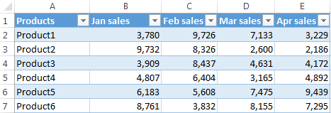
If you'd rather have alternate row shading only, without the table functionality, you can easily convert the table back to a usual range. To do this, select any cell within your table, right click and choose Convert to Range from the context menu.
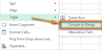
Note. After performing the table-to-range transformation, you won't get the automatic color banding for newly added rows. Another disadvantage is that if you sort the data, your color bands will travel with the original rows and your nice zebra stripe pattern will get distorted.
As you can see, converting a range to table is a very easy and quick way of highlighting alternate rows in Excel. But what if you want a bit more?
How to choose your own colors of row stripes
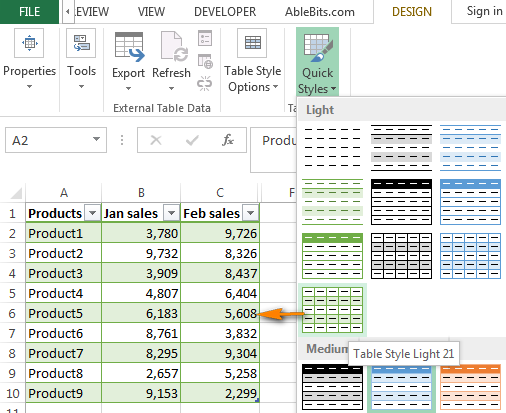
If you are not happy with the default blue and white pattern of an Excel table, you have plenty more patterns and colors to choose from. Just select your table or any cell within the table, switch to the Design tab > Table Styles group and select the colors of your liking.
You can use the arrow buttons to scroll through the available table styles or click the More button ![]() to view them all. When you hover the mouse cursor over any style, it is immediately reflected to your table and you can see how your banded rows would look like.
to view them all. When you hover the mouse cursor over any style, it is immediately reflected to your table and you can see how your banded rows would look like.
How to highlight a different number of rows in each zebra line
In case you want to highlight a different number of rows in each stripe, e.g. shade 2 rows in one color and 3 in another, then you will need to create a custom table style. Assuming that you have already converted a range to table, perform the following steps:
- Navigate to the Design tab, right click on the table style you want to apply and choose Duplicate.

- In the Name box, enter a name of your table style.
- Select "First Row Stripe" and set the Stripe Size to 2, or to some other number you want.
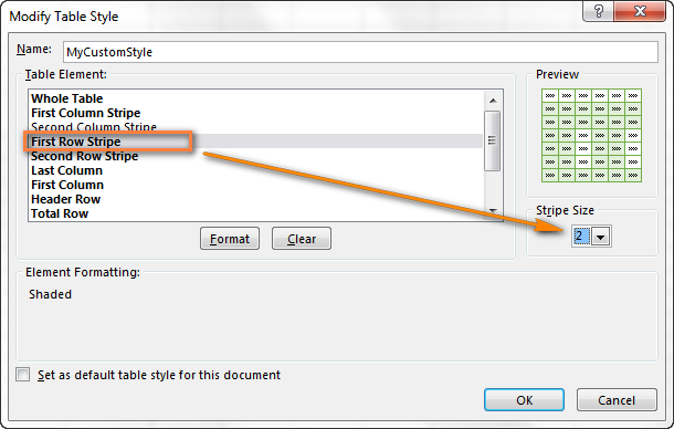
- Select "Second row stripe" and repeat the process.
- Click OK to save your custom style.
- Apply the newly created style to your table by selecting it from the Table Styles gallery. Your custom styles are always available at the top of the gallery under Custom.

Note: Custom table styles are stored only in the current workbook and therefore are not available in your other workbooks. To use your custom table style as the default table style in the current workbook, select the "Set as default table style for this document" check box when creating or modifying the style.

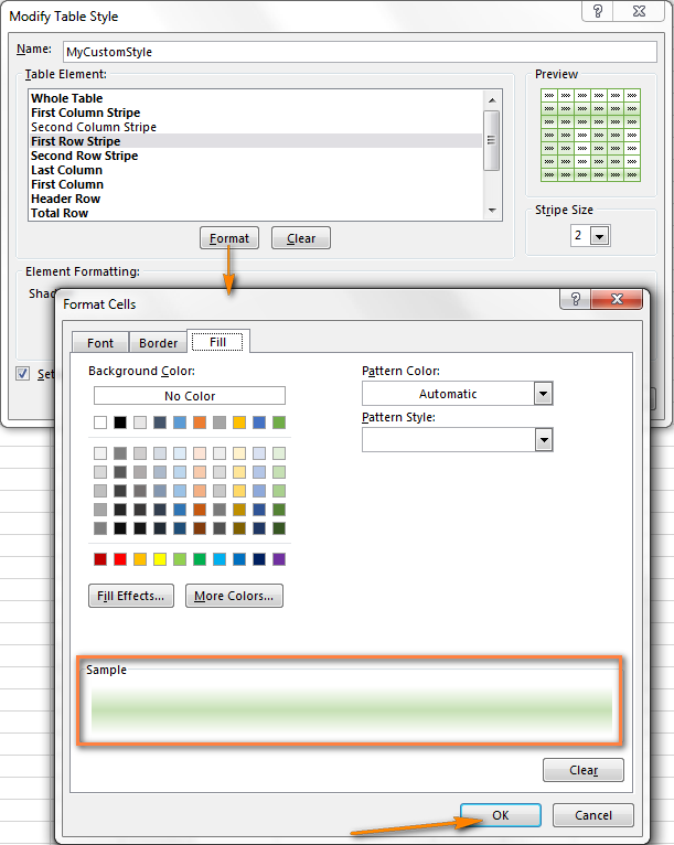
If you are not happy with the style you created, you can easily modify it by right-clicking your custom style in the Styles Gallery and choosing Modify from the context menu. And here you have plenty of room for your creativity! You can set any Font, Border, and Fill styles on the corresponding tabs, even choose gradient stripe colors, as you see in the screenshot below : )
Remove alternate rows color in Excel with a click
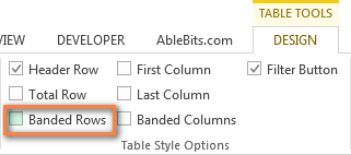
If you no longer want to have color banding in your Excel table, you can remove them literally in a single click. Select any cell in your table, go to the Design tab and uncheck the Banded rows option.
As you see, Excel's predefined table styles provide a wealth of features to alternate color rows in your worksheets and create custom banded rows styles. I believe they will suffice in many situations, though if you want something special, e.g. shading entire rows based on a change of value, then you will need to use conditional formatting.
Alternate row color shading using Excel conditional formatting
It goes without saying that conditional formatting is a bit trickier that Excel table styles we have just discussed. But it has one undisputable benefit - it allows more room for your imagination and lets you zebra stripe your worksheet exactly as you want it is each particular case. Further on in this article, you will find a few examples of Excel formulas for alternating row colors:
- Shade every other row
- Shade groups of rows with different colors
- Highlight rows using 3 colors
- Alternate rows based on value change
Highlight every other row in Excel using conditional formatting
We are going to start with a very simple MOD formula that highlights every other row in Excel. In fact, you can achieve exactly the same result using Excel Table styles, but the main benefit of conditional formatting is that it works for ranges as well, meaning that your color banding will remain intact as you sort, insert or delete rows in a range of data to which your formula applies.
You create a conditional formatting rule in this way:
- Select the cells you want to shade. To apply the color banding to the entire worksheet, click the Select All button in the top left-hand corner of your spreadsheet.

- Switch to the Home tab > Styles group and click Conditional Formatting > New Rule...
- In the New Formatting Rule window, choose "Use formula to determine which cells to format" option and enter this formula:
=MOD(ROW(),2)=0
- Then click the Format button, switch to the Fill tab and select the background color that you want to use for the banded rows.
At this point, the selected color will appear under Sample. If you are happy with the color, click OK.
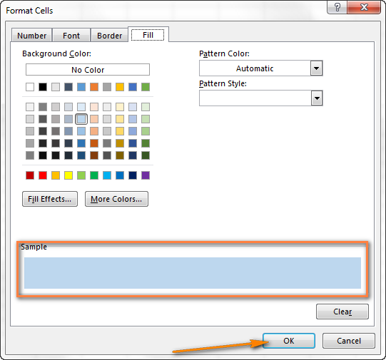
- This will bring you back to the New Formatting Rule window, and you click OK one more time to apply to color to every other of the selected rows.
And here's how the result looks like in my Excel 2013:

If you'd rather have 2 different colors instead of white lines, then create a second rule using this formula:
=MOD(ROW(),2)=1And now you have odd and even rows highlighted with different colours:

That was pretty easy, wasn't it? And now I'd like to briefly explain the syntax of the MOD function because we are going to use it in other a bit more complex examples.
The MOD function returns the remainder rounded to the nearest integer after the number is divided by the divisor.
For example, =MOD(4,2) returns 0, because 4 is divided by 2 evenly (without remainder).
Now, let's see what exactly our MOD function, one that we've used in the above example, does. As you remember we used a combination of the MOD and ROW functions: =MOD(ROW(),2) The syntax is simple and straightforward: the ROW function returns the row number, then the MOD function divides it by 2 and returns the remainder rounded to the integer. When applied to our table, the formula returns the following results:
| Row No. | Formula | Result |
|---|---|---|
| Row 2 | =MOD(2,2) | 0 |
| Row 3 | =MOD(3,2) | 1 |
| Row 4 | =MOD(4,2) | 0 |
| Row 5 | =MOD(5,2) | 1 |
Do you see the pattern? It's always 0 for even rows and 1 for odd rows. And then we create the conditional formatting rules telling Excel to shade odd rows (where the MOD function returns 1) in one color and even rows (that have 0) in another color.
Now that you know the basics, let's look into more sophisticated examples.
How to alternate groups of rows with different colors
You can use the following formulas to shade a fixed number of rows, regardless of their content:
Odd row shading, i.e. highlight the 1st group and every other group:
=MOD(ROW()-RowNum,N*2)+1<=N
Even row shading, i.e. highlight the 2nd group and all even groups:
=MOD(ROW()-RowNum,N*2)>=N
Where RowNum is a reference to your first cell with data and N is the number of rows in each banded group.
Tip: If you want to highlight both even and odd groups, then simply create 2 conditional formatting rules with both of the above formulas.
You can find a few examples of formula usage and the resulting color banding in the following table.
| To color every 2 rows, starting from the 1st group. The data starts in row 2. | =MOD(ROW()-2,4)+1<=2 |
 |
|---|---|---|
| To color every 2 rows, starting from the 2nd group. The data starts in row 2. | =MOD(ROW()-2,4)>=2 |
 |
| To color every 3 rows, starting from the 2nd group. The data starts in row 3. | =MOD(ROW()-3,6)>=3 |
 |
How to shade rows with 3 different colors
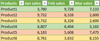
If you think your data will look better with rows shaded in three different colors, then create 3 conditional formatting rules with these formulas:
To highlight 1st and every 3rd row =MOD(ROW($A2)+3-1,3)=1
To highlight 2nd, 6th, 9th etc. =MOD(ROW($A2)+3-1,3)=2
To highlight 3rd, 7th, 10th etc. =MOD(ROW($A2)+3-1,3)=0
Remember to replace A2 with a reference to your first cell with data.
The resulting table will look similar to this in your Excel:
How to alternate row colors based on a value change
This task is similar to the one we discussed a moment ago - shading groups of rows, with the difference that there may be a different number of rows in each group. I believe, this will be easier to understand from an example.
Suppose, you have a table containing data from different sources, e.g. regional sales reports. What you want is shade the first group of rows related to the first product in Color 1, the next group related to the second product in Color 2 and so on. Column A listing the product names may serve as the key column or unique identifier.

To alternate row shading based on change of value, you'd need a bit more complex formula and an additional column:
- Create an additional column over the right side of your worksheet, say column F. You will be able to hide this column later.
- Enter the following formula in cell F2 (assuming that row 2 is your first row with data) and then copy it across the entire column:
=MOD(IF(ROW()=2,0,IF(A2=A1,F1, F1+1)), 2)The formula will fill down column F with blocks of 0 and 1, every new block staring with the Product name change.

- And finally, create a conditional formatting rule using the formula
=$F2=1. You can add a second rule=$F2=0if you want a second color to alternate blocks of rows, as shown in the screenshot:
Alternating column colors in Excel (banded columns)
In fact, shading columns in Excel is pretty much similar to alternating rows. If you have understood all of the above, this part is going to be a piece of pie for you : )
You can apply shading to columns in Excel by using either:
Alternate column colors in Excel with table styles
- You start with converting a range to a table (Ctrl+T).
- Then switch to the Design tab, remove a tick from Banded rows and select Banded columns instead.

- Voila! Your columns are shaded with the default table colors.

In case you'd like prettier colors, you are free to choose any other pattern from the Table Styles Gallery.
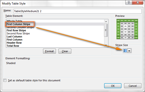
If you want to shade a different number of columns in each stripe, then create a duplicate of an existing table style of your choosing, exactly as described here. The only difference is that you choose "First Colum Stripe" and "Second Colum Stripe" instead of the corresponding row stripes.
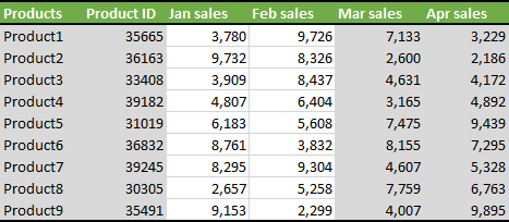
And this is how your custom column bands may look like in Excel:
Alternating column colors with conditional formatting
The formulas to apply color banding to alternate columns in Excel are very similar to the ones we've used for shading alternate rows. You just need to use the MOD function in conjunction with the COLUMN function rather than ROW. I will name but a few in the table below and I'm sure you will easily convert other "row formulas" to "column formulas" by analogy.
| To color every other column | =MOD(COLUMN(),2)=0and/or =MOD(COLUMN(),2)=1 |
 |
|---|---|---|
| To color every 2 columns, starting from the 1st group | =MOD(COLUMN()-1,4)+1<=2 |
 |
| To shade columns with 3 different colors | =MOD(COLUMN()+3,3)=1=MOD(COLUMN()+3,3)=2=MOD(COLUMN()+3,3)=0 |
 |
Hopefully, now you won't have any problems with applying color banding in Excel to make your worksheets handsome and more readable. If you want to alternate row or column colors in some other way, don't hesitate to leave me a comment and we will figure this out together. Thank you for reading!
 by
by
78 comments
Excellent information, thanks.
I am wanting banded rows without a table so I'm using conditional formatting with the MOD function. I don't want the empty rows below my data to be banded, if there is no data in column A the whole row stays unformatted. But if I enter data in column a the row formats. Does that make sense?
Hi! If I understand you correctly, you can create another conditional formatting rule that sets the default format for rows that have no data. Please have a look at these guidelines for the formatting of rows: Apply multiple rules to same cells.
I have a table as such:
Ali. $1.20
Ali: $1.80
Ali: $1.00
Steven: $2.00
Steven: $4.00
Steven: $5.00
Steven: $7.00.
Mary: $4.00
Mary: $2.00
Mary: $6.00
Mary: $7.00
Mary: $8.00
The range differs every month. Ali’s range may be more or less and Steven’s range may be more or less and Mary’s range may be more or less
I need to highlight these ranges alternately.
Highlight Ali first, leave Steven blank and highlight Mary again. Please help. Thank u
Thank u
Hi! Using these instructions, you can highlight a row in color based on the data in the first column: How to change the row color based on a cell value in Excel.
I have a table with 3 different states in it that I need to have different colors for each state and also needs to be alternating colors in each state. Every week there will be additions or deletions. Is there a way to do this where it will do two colors for each state based upon the state name which is listed in one of the columns?
Hi! You need to create a separate conditional formatting rule for each color. You can use this guide: Excel conditional formatting formulas based on another cell.
hello. I am super impressed and just wanted to do a shout out at your amazing skills. I was asked to do alternating rows for groups of similar data and your formula is pretty simple and it WORKS. good tips: 2 thumbs up.
Hi,
I am using =MOD(ROW(),2)=0 to shade alternating rows. However the shaded rows override any shading or fill that i apply manually. I would like to highlight yellow as I am reviewing a document and this only works on the non shaded rows. I have looked at using AND(=MOD(ROW(),2)=0,CELL('color',INDEX(ROW(),COLUMN())) but CELL('color') only works for negative cell values, whereas i have text, numbers and empty cells I would like it to apply to. Anyone else come across this one?
Many thanks.
Hi!
The CELL function cannot identify the color of a cell. You must use a custom function and Visual Basic for that. Maybe you can use user-defined function GetCellColor(). You can find its detailed description and examples in this article: How to sum and count cells by color in Excel.
I want to color duplicate rows different colors. I am using =COUNTIF but it makes all the duplicates the same color. Can I make a row that has all AAAAs in a cell green and then all BBBBs are red? There is a ton of data so I am searching for duplicate values not specific values. Thanks!
Hello!
Create a separate conditional formatting rule with its own color for each type of duplicate.
Odd row shading, i.e. highlight the 1st group and every other group:
=MOD(ROW()-RowNum,N*2)+1<=N
Why in the given formula we have multiplied N by *2 ?
What is the reason?
Is there a formula to highlight a row when you mouseover?
Hi,
I need to give alternate merged rows different color along with its non merged adjacent columns. Example A1:A2 , A3:A4 , A5:A6 , A7:A8 are merged. But B1:B8 are not merged. I want all the columns of rows (1,2), (5,6) blue colour and the other sets white
Hi,
I have excel template and fill the data from database. There could any number of data in excel. Its first column merge on the basis of duplicate data. I want to do setting in the excel template for alternate merge rows coloring. Please help me to do this.
Note :- I don't know the number of rows.
How can I shade alternate rows but only that display data, the reminder rows must stay without shade? Thanks
Hello Gustavo!
I’m sorry but your task is not entirely clear to me. Explain what you mean by "reminder rows"? It’ll help me understand it better and find a solution for you. Thank you.
Hi,
As beginner in excel functions, please I need your help:
I have this question:
How to use highlight Mod function for alternating shading in one chosen row easily?
Is it possible to mix MOD function with other condition in one formula for this row.
For example use function AND : example in the first column in this chosen row is inserted value (for example 1 function : = 1) , how to u use function MOD(column) in this row?
Thank for youur help
Regards
Jerry
Thanks for these great tips! I found exactly what I needed ^_^
how can I shade columns in this pattern-- black, white, red, white, black, white, red, white?
the easiest way I know is by intorducing the following formula as a new rule in conditional formating: = =indirect("A"&ROW())="Product1" and ofcourse choose a color for this selection. I hope it hels as the examples above are too complicated or not selective enough.
Thanks..
I want to know all excel formula
The results are not bad but,
sorry, always to use them, my page brake for printing is one line higher as it shall be :-(
How to install colored lines in changing with noncolored lines under the page brake rules?
To correct all 2000 lines to move several page brakes is not fine.
Hi,
I want to color upper row, when I am in down cell
Hello,
Please try using a VBA macro. We are always ready to help you, but we do not cover the programming area (VBA-related questions).
You may try to find the solution in VBA sections on mrexcel.com or excelforum.com.
Sorry we can’t assist you better.