This tutorial focuses on various ways to calculate times in Excel. You will find a few useful formulas to add and subtract times, calculate time difference, or elapsed time, and more.
In the last week's article, we had a close look at the specificities of Excel time format and capabilities of basic time functions. Today, we are going to dive deeper into Excel time calculations and you will learn a few more formulas to efficiently manipulate times in your worksheets.
How to calculate time difference in Excel (elapsed time)
To begin with, let's see how you can quickly calculate elapsed time in Excel, i.e. find the difference between a beginning time and an ending time. And as is often the case, there is more than one formula to perform time calculations. Which one to choose depends on your dataset and exactly what result you are trying to achieve. So, let's run through all methods, one at a time.
Formula 1. Subtract one time from the other
As you probably know, times in Excel are usual decimal numbers formatted to look like times. And because they are numbers, you can add and subtract times just as any other numerical values.
The simplest and most obvious Excel formula to calculate time difference is this:
Depending on you data structure, the actual time difference formula may take various shapes, for example:
| Formula | Explanation |
=A2-B2 |
Calculates the difference between the time values in cells A2 and B2. |
=TIMEVALUE("8:30 PM") - TIMEVALUE("6:40 AM") |
Calculates the difference between the specified times. |
=TIME(HOUR(A2), MINUTE(A2), SECOND(A2)) - TIME(HOUR(B2), MINUTE(B2), SECOND(B2)) |
Calculates the time difference between values in cells A2 and B2 ignoring the date difference, when the cells contain both the date and time values. |
Remembering that in the internal Excel system, times are represented by fractional parts of decimal numbers, you are likely to get the results similar to this:

The decimals in column D are perfectly true but not very meaningful. To make them more informative, you can apply custom time formatting with one of the following codes:
| Time code | Explanation |
| h | Elapsed hours, display as 4. |
| h:mm | Elapsed hours and minutes, display as 4:10. |
| h:mm:ss | Elapsed hours, minutes and seconds, display as 4:10:20. |
To apply the custom time format, click Ctrl + 1 to open the Format Cells dialog, select Custom from the Category list and type the time codes in the Type box. Please see Creating a custom time format in Excel for the detailed steps.
And now, let's see how our time difference formula and time codes work in real worksheets. With Start times residing in column A and End times in column B, you can copy the following formula in columns C though E:
=$B2-$A2
The elapsed time is displayed differently depending on the time format applied to the column:

Note. If the elapsed time is displayed as hash marks (#####), then either a cell with the formula is not wide enough to fit the time or the result of your time calculations is a negative value.
Formula 2. Calculating time difference with the TEXT function
Another simple technique to calculate the duration between two times in Excel is using the TEXT function:
- Calculate hours between two times:
=TEXT(B2-A2, "h") - Return hours and minutes between 2 times:
=TEXT(B2-A2, "h:mm") - Return hours, minutes and seconds between 2 times:
=TEXT(B2-A2, "h:mm:ss")

Notes:
- The value returned by the TEXT function is always text. Please notice the left alignment of text values in columns C:E in the screenshot above. In certain scenarios, this might be a significant limitation because you won't be able to use the returned "text times" in other calculations.
- If the result is a negative number, the TEXT formula returns the #VALUE! error.
Formula 3. Count hours, minutes or seconds between two times
To get the time difference in a single time unit (hours ,minutes or seconds), you can perform the following calculations.
Calculate hours between two times:
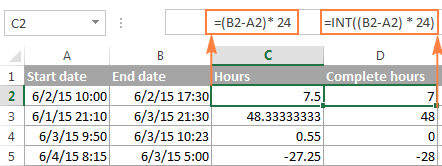
To present the difference between two times as a decimal number, use this formula:
Supposing that your start time is in A2 and end time in B2, you can use a simple equation B2-A2 to calculate the difference between two times, and then multiply it by 24, which is the number of hours in one day:
=(B2-A2) * 24
To get the number of complete hours, use the INT function to round the result down to the nearest integer:
=INT((B2-A2) * 24)
Total minutes between two times:
To calculate the minutes between two times, multiply the time difference by 1440, which is the number of minutes in one day (24 hours * 60 minutes = 1440).
As demonstrated in the following screenshot, the formula can return both positive and negative values, the latter occur when the end time is less than the start time, like in row 5:
=(B2-A2)*1440

Total seconds between times:
To get the total seconds between two times, you multiply the time difference by 86400, which is the number of seconds in one day (24 hours * 60 minutes * 60 seconds = 86400).
In our example, the formula is as follows:
=(B2-A2)* 86400
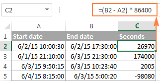
Note. For the results to display correctly, the General format should be applied to the cells with your time difference formula.
Formula 4. Calculate difference in one time unit ignoring others
To find the difference between 2 times in a certain time unit, ignoring the others, use one of the following functions.
- Difference in hours, ignoring minutes and seconds:
=HOUR(B2-A2) - Difference in minutes, ignoring hours and seconds:
=MINUTE(B2-A2) - Difference in seconds, ignoring hours and minutes:
=SECOND(B2-A2)
When using Excel's HOUR, MINUTE and SECOND functions, please remember that the result cannot exceed 24 for hours and 60 for minutes and seconds.

Note. If the end time is less than the start time (i.e. the result of the formula is a negative number), the #NUM! error is returned.
Formula 5. Calculate elapsed time from a start time to now
In order to calculate how much time has elapsed since the start time to now, you simply use the NOW function to return today's date and the current time, and then subtract the start date and time from it.
Supposing that the beginning date and time is in call A2, the formula below returns the following results, provided you've applied an appropriate time format to column B, h:mm in this example:
=NOW()-A2

In case the elapsed time exceeds 24 hours, use one of these time formats, for example d "days" h:mm:ss like in the following screenshot:

If your starting points contain only time values without dates, you need to use the TIME function to calculate the elapsed time correctly. For example, the following formula returns the time elapsed since the time value in cell A2 up to now:
=TIME(HOUR(NOW()), MINUTE(NOW()), SECOND(NOW())) - A2
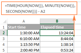
Note. The elapsed time is not updated in real-time, it refreshes only when the workbook is reopened or recalculated. To force the formula to update, press either Shift + F9 to recalculate the active spreadsheet or hit F9 to recalculate all open workbooks.
Formula 5. Display time difference as "XX days, XX hours, XX minutes and XX seconds"
This is probably the most user-friendly formula to calculate time difference in Excel. You use the HOUR, MINUTE and SECOND functions to return corresponding time units and the INT function to compute the difference in days. And then, you concatenate all these functions in a single formula along with the text labels:
=INT(B2-A2) & " days, " & HOUR(B2-A2) & " hours, " & MINUTE(B2-A2) & " minutes and " & SECOND(B2-A2) & " seconds"

To instruct your Excel time difference formula to hide zero values, embed four IF functions into it:
=IF(INT(B2-A2)>0, INT(B2-A2) & " days, ","") & IF(HOUR(B2-A2)>0, HOUR(B2-A2) & " hours, ","") & IF(MINUTE(B2-A2)>0, MINUTE(B2-A2) & " minutes and ","") & IF(SECOND(B2-A2)>0, SECOND(B2-A2) & " seconds","")
The syntax may seem excessively complicated, but it works :)

Alternatively, you can calculate time difference by simply subtracting the start time from the end time (e.g. =B2-A2), and then apply the following time format to the cell:
d "days," h "hours," m "minutes and" s "seconds"
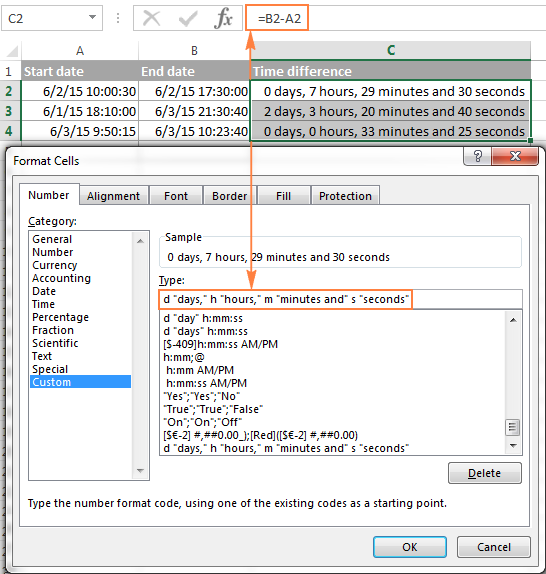
An advantage of this approach is that your result would be a normal time value that you could use in other time calculations, while the result of the complex formula discussed above is a text value. A drawback is that the custom time format cannot distinguish between zero and non-zero values and ignore the latter. To display the result in other formats, please see How to show time over 24 hours, 60 minutes, 60 seconds.
How to calculate and display negative times in Excel
When calculating the time difference in Excel, you may sometimes get the result as ###### error because the difference is a negative time. But is there a way to show negative times properly in Excel? Of course, there is a way, and even more than one :)
Method 1. Change Excel Date System to 1904 date system
The fastest and easiest way to display negative time normally (with a minus sign) is switching to the 1904 date system. To do this, click File > Options > Advanced, scroll down to the When calculating this workbook section and put a tick in the Use 1904 date system box.

Click OK to save the new settings, and from now on negative times will be displayed correctly, like negative numbers:

Method 2. Calculate negative time in Excel with formulas
Is changing Excel's default Date System is not an option, then you can force negative times to display properly using one of the following formulas:
=IF(A2-B2>0, A2-B2, "-" & TEXT(ABS(A2-B2),"h:mm"))
=IF(A2-B2>0, A2-B2, TEXT(ABS(A2-B2),"-h:mm"))
Both formulas check if the time difference (A2-B2) is greater than 0, and if it is they return that difference. If the time difference is less than zero, the first formula calculates the absolute difference and concatenates the minus sign. The second formula yields exactly the same result by using a negative time format "-h::mm".

Note. Please keep in mind that unlike the first method that treats negative times as negative numeric values, the result of the TEXT function is always a text string that cannot be used in calculations or other formulas.
Adding and subtracting time in Excel
Basically, there are 2 ways to add and subtract time in Excel:
- Using the TIME function
- Using arithmetic calculations based on the number of hours (24), minutes (1440) and seconds (86400) in one day
The TIME(hour, minute, second) function makes Excel time calculations really easy, however it does not allow adding or subtracting more than 23 hours, or 59 minutes, or 59 seconds. If you are working with bigger time intervals, then use one of the arithmetic calculations demonstrated below.
How to add or subtract hours to time in Excel
To add hours to a given time in Excel, you can use one the following formulas.
TIME function to add under 24 hours
For example, if your start time is in cell A2, and you want to add 2 hours to it, the formula is as follows:
=A2 + TIME(2, 0, 0)
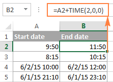
Note. If you try adding more than 23 hours with the TIME function, the specified hours will be divided by 24 and the remainder will be added to the start time value. For example, if you try to add 25 hours to "6/2/2015 10:00 AM" (cell A4) using the formula =A4 + TIME(25, 0, 0), the result will be "06/02/2015 11:00", i.e. A4 + 1 hour.
Formula to add any number of hours (under or over 24 hours)
The following formula has no limitations to the number of hours you want to add:
For example, to add 28 hours to the start time in cell A2, enter the following formula:
=A2 + (28/24)

To subtract hours from a given time, you use analogous formulas, and just replace "+" with the minus sign:
For example, to subtract 3 hours from the time in cell A2, either of the following formulas will do:
=A2-(3/24)
=A2-TIME(3,0,0)
To subtract more than 23 hours, use the first one.
How to add / subtract minutes to time in Excel
To add minutes to a given time, employ the same techniques that we've just used for adding hours.
To add or subtract under 60 minutes
Use the TIME function and supply the minutes you want to add or subtract in the second argument:
And here are a couple of real-life formulas to calculate minutes in Excel:
To add 20 minutes to the time in A2: =A2 + TIME(0,20,0)
To subtract 30 minutes from the time in A2: =A2 - TIME(0,30,0)
To add or subtract over 60 minutes
In your calculation, divide the number of minutes by 1440, which is the number of minutes in a day, and add the quotient to the start time:
To subtract minutes from time, simply replace plus with the minus sign. For example:
To add 200 minutes: =A2 + (200/1440)
To subtract 300 minutes: =A2 -(300/1440)

How to add / subtract seconds to a given time
Second calculations in Excel are done in a similar fashion.
To add under 60 seconds to a given time, you can use the TIME function:
To add more than 59 seconds, use the following formula:
To subtract seconds, utilize the same formulas with the minus sign (-) instead of plus (+).
In your Excel worksheets, the formulas may look similar to these:
To add 30 seconds to A2: =A2 + TIME(0,0,31)
To add 1200 seconds to A2: =A2 + (1200/86400)
To subtract 40 seconds from A2: =A2 - TIME(0,0,40)
To subtract 900 seconds from A2: =A2 - (900/86400)
How to sum time in Excel
The Excel sum time formula is the usual SUM function, and applying the proper time format to the result is what does the trick.
Supposing you have a few project times in column B and you want to add them up. You write a simple SUM formula like the one below and get the result in the default format such as hh:mm:ss.
=SUM(B2:B4)
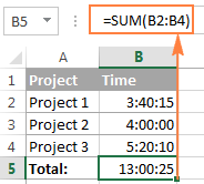
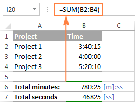
In some cases the default time format works just fine, but sometimes you may want more, for example to display the total time as minutes and seconds, or seconds only. The good news is that no other calculations are required, all you have to do is apply custom time format to the cell with the SUM formula.
Right click the cell and select Format Cells in the context menu, or press Ctrl + 1 to open the Format Cells dialog box. Select Custom from the Category list and type one of the following time formats in the Type box:
- To display total time as minutes and seconds: [m]:ss
- To display total time as seconds: [ss]
The result will look as follows:
How to sum over 24 hours in Excel
In order to add up more than 24 hours, you use the same SUM formula as discussed above, and apply one of the following time formats to the cell:
| Format | Displays as | Explanation |
| [h]:mm | 30:10 | Hours and minutes |
| [h]:mm:ss | 30:10:20 | Hours, minutes and seconds |
| [h] "hours", mm "minutes", ss "seconds" | 30 hours, 10 minutes, 20 seconds | |
| d h:mm:ss | 1 06:10:20 | Days, hours, minutes and seconds |
| d "day" h:mm:ss | 1 day 06:10:20 | |
| d "day," h "hours," m "minutes and" s "seconds" | 1 day, 6 hours, 10 minutes and 20 seconds |
To see how these custom time formats may look like in your Excel worksheet, please have a look at the screenshot below, where the same SUM formula is entered in cells A9 to A13:
=SUM($B$2:$B$4)
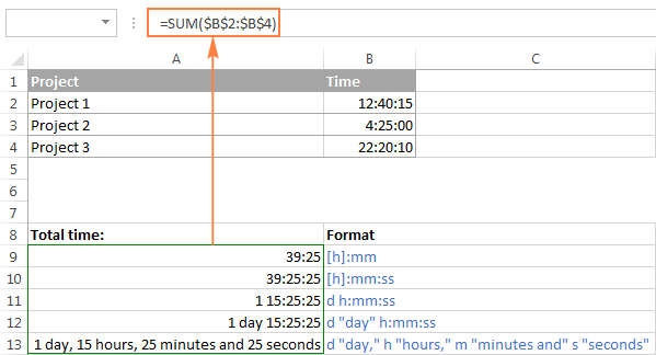
Note. The above custom time formats work for positive values only. If the result of your time calculations is a negative number, e.g. when you are subtracting a bigger time from a smaller time, the result will be displayed as #####. To display negative times differently, please see custom format for negative time values.
Also, please keep in mind that the time format applied to a cell changes only the display presentation without changing the cell's value. For example, in the screenshot above, cell A13 looks like text, but in fact it's a usual time value, which is stored as a decimal in the internal Excel system. Meaning, you are free to refer to that cell in other formulas and calculations.
For more information, please see How to calculate and show over 24 hours, 60 minutes, 60 seconds.
Date & Time Formula Wizard - quick way to calculate times in Excel
Now that you know a bunch of different formulas to add and subtract times in Excel, let me show you the tool that can do it all. Okay, almost all :)
Here comes Ablebit's Date & Time Formula Wizard for Excel:

In the Date & Time Wizard dialog window, you switch to the Add or Subtract tab, depending on which operation you want to perform, and do the following:
- Click the Show time fields link in the left part of the window.
- Supply values or cell references for the formula arguments. As you fill in the argument boxes, the wizard builds the formula in the selected cell.
- When finished, click the Insert Formula
That's it! For example, this is how you can add the specified number of hours, minutes and seconds to the time in A4:
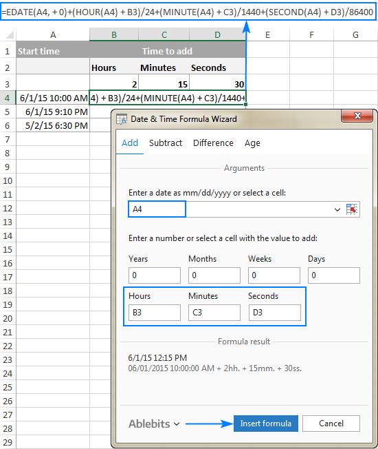
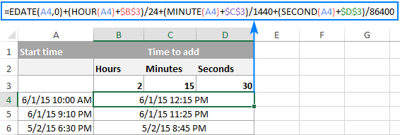
If you need to copy the formula to other cells, fix all references except the cell containing the original time (A4) with the $ sign like shown in the screenshot below (by default, the wizard always uses relative references). Then double-click the fill handle to copy the formula down the column and you are good to go!
Besides time calculations, the wizard can also add and subtract dates, get the difference between two dates, and calculate age from the birthdate.
If you are curious to try this tool in your own worksheets, you are welcome to download the evaluation version of our Ultimate Suite below.
This is how you calculate time in Excel worksheets. To learn other ways to manipulate dates and times in Excel, I encourage you to check out the resources at the end of this article. I thank you for reading and hope to see you on our blog next week!
Available downloads
Excel Time Calculations - formula examples (.xlsx file)
Ultimate Suite - trial version (.exe file)
 by
by
1042 comments
Is there a way to subtract either different amounts of business hours from a date and time, excluding holidays, and have the result calculated to the hour? For example, I have a task that is due by 9am on 05/27/2025. I need to subtract 18 business hours (a 9-hour work day, starting at 8am and ending at 5pm). Memorial Day is the day before (05/26/2025), and the weekend is the 2 days before that, so my cancelation date and time should be 9am on 05/22/2025. Same example, but subtracting 24 business hours. The cancelation time should be 12 noon on 05/21/2025. My data is as such:
start date, displayed just as the date: d2
start time, displayed just as the time: e2
combined start date and time (if needed): f2
cancelation hours: ae2
holidays for current year: $BP$2:$BP$13
Any help would be greatly appreciated!
J
Hello Jenn!
The number of working days to subtract from the date and time (9am on 05/27/2025) can be calculated using the INT function.
Subtract these working days using the formula WORKDAY.INTL. Read more: Calculating weekdays in Excel - WORKDAY and NETWORKDAYS functions.
The number of extra hours to subtract from the date and time (9am on 05/27/2025) can be calculated using the MOD function.
If the number of extra hours is greater than 0, subtract one more working day. Subtract Extra hours from the end time of the working day.
=IF(MOD(A2,9)/24>0, WORKDAY.INTL(F2,-(INT(A2/9+1)),1,B2:B6)+TIME(17,0,0)-MOD(A2,9)/24, WORKDAY.INTL(F2,-INT(A2/9),1,B2:B6)+MOD(F2,1))
A2=24
F2=05/27/2025 9:00:00 AM
B2:B6 - holidays
Hi, Alexander! Thank you for this formula! It works perfectly for an 18 business hour cancelation, but not for a 24 business hour cancelation. Is there a way to modify the formula based on another cell containing either 18 or 24? Or, a nested if/then statement inside the current formula?
Hi! Explain why you think the formula is not working correctly. The formula returns the correct result 21/05/2025 11:00.
Unless my calculations are incorrect, the formula should return the result of 05/21/2025 at 12-noon, not 11am.
05/27/2025 9 am to 8 am: 1 hour (23 remaining)
05/26/2025 Holiday
05/25/2025 Sunday
05/24/2025 Saturday
05/23/2025 5pm to 8 am: 9 hours (14 remaining)
05/22/2025 5pm to 9 am: 8 hours (5 remaining)
05/21/2025 5pm to 12 noon: 5 hours (0 remaining)
Hi! It looks like your problem cannot be solved with a single Excel formula.
Could you at least give me a direction? Why does it work for 18 hours, but not for 24? What data would I need and what functions would work best?
I am trying to calculate how many hours worked within a start time and end time. For example, punch in time is 4:30 AM and punch time is 1:00 pm. I want to calculate how hours worked in between 12:00 PM and 3:00 PM.
Hello Brittany! I recommend reading the comments below where the exact same question was asked. Try this formula:
=(B1-A1)-IF(C1>A1,C1-A1,0)-IF(B1>C2,B1-C2,0)
B1=12:00 PM
A1=3:00 PM
C1 and C2 - statr and end time
hello i have a request
i want to calculate the time interval between 22:00 until 06:00 for example even if i write 17:00 until tomorrow 07:00 i want the formula to calculate only the time between 22:00 until 06:00
no professor i meant i want to calculate only the time from 22:00 to 06:00 even if for example the entr is given earlier and the exit is given later for example from 22:00 to 06:00 is 8 hours long and if i make another entry from 21:00 and the exit at 07:00 i want the formula to calculate only from 22:00 to 06:00
Hi! Have you checked how this formula works? It returns at 8 hours, according to your entry at 21:00 and exit at 07:00.
Hi! If I understand your task correctly, try the following formula:
=TIME(8,0,0)-IF(C1>A1,C1-A1,0)-IF(B1>C2,B1-C2,0)
A1= 22:00
B1= 06:00
C1= 17:00
C2= 07:00
Hi. I'm trying to calculate my work hours and am struggling. I'm a vendor and have different requirements for different customers. Customer A pays me a different rate before 6 am and after 6pm, and customer B pays me that same rate before 8 am and after 5 pm, Monday through Friday. They both pay the same rate on Saturdays and Sundays all day. So, my data looks like this:
Column A | Column B | Column C | Column D | Column E | Column F
Customer | Date | Day | Start Time | End Time | Duration
A | 02/06/2025 | Thursday | 5:00 am | 11:00 am | 6 hours
B | 02/06/2025 | Thursday | 7:00 am | 11:00 am | 4 hours
A | 02/06/2025 | Thursday | 6:00 pm | 11:00 pm | 5 hours
B | 02/06/2025 | Thursday | 5:00 pm | 11:00 pm | 6 hours
A | 02/09/2025 | Sunday | 8:00 am | 8:00 pm | 12 hours
B | 02/09/2025 | Sunday | 8:00 am | 5:00 pm | 9 hours
I need to have one formula that will take into account which customer is paying me, the day of the week, and if the start time is outside of their business hours so I can calculate my income for each task. In the above example,
Row 1: I will be paid $65 from 5am to 6am, and $60 from 6am to 11 am.
Row 2: I will be paid $65 from 7am to 8am, and $60 from 8am to 11 am.
Row 3: I will be paid $65 from 6pm to 11pm.
Row 4: I will be paid $65 from 5pm to 11 pm.
Row 5: I will be paid $65 from 8am to 8pm.
Row 6: I will be paid $65 from 8am to 5pm.
Thanks for your help!
J
Hi! Your request goes beyond the advice we provide on this blog. This is a complex solution that cannot be found with a single formula. If you have a specific question about the operation of a function or formula, I will try to answer it.
I tried the following format:
d "days," h "hours," m "minutes and" s "seconds"
However the moment the time difference is over 30 days (it seems) it does not work.
Hi! You can find the answer to your question in this article: Excel DATEDIF to calculate date difference in days, weeks, months or years.
Please Help me
In time 06.00AM, Tiffen Time 9.00AM to 9.30AM, Lunch Time 2:30PM to 3.00PM
Question: 01
In time 06.00AM, Out Time 01.00PM
Working Time ? without tiffen Time.
Question 02.
Intime 06.00AM, Out Time 2:52PM
Working Time = ? without tiffen Time and lunch time.
Hi! To calculate the number of working hours including Tiffen Time and Lunch Time, you can use the SUMIFS formula.
To do this, write a sequence of time values in column A with an interval of 30 minutes. For example, 06:00, 06:30, 07:00, and so on. In column B, write 1 if it is a working time and 0 if it is not. For example, the times 09:30 and 15:00 correspond to 0.
If In Time and Out Time are written in C1 and C2, try this SUMIFS formula:
=SUMIFS(B1:B25,A1:A25,">="&C1,A1:A25,"<="&C2)/2
Hello, your article helped me a lot, but I'm still struggling with time zones.
I need to calculate time crossing time zones, in where the time zones may change depending on the trip. So far I have the following columns:
C1 (Start Time H:mm AM/PM) | D1 (End Time H:mm AM/PM) | E1 (Time Zone Adjustment* #) | F1 (Total Time H:mm)
*Time Zone Adjustment is a single number 0 through 4, as we are based in Alaska and frequently travel to the East Coast. AK Time is 0, Pacific Time is 1, Mountain 2, Central 3, and Eastern 4.
I have a need to figure out how much time my employees spend traveling so that we can calculate Travel Compensation Time. My idea is to enter each leg of the trip per line and calculate the total via SUM.
Thank you in advance!
Hello Samie!
If I understand the question correctly, to convert a number to a hours, use the TIME function. You can also use these instructions: How to convert numbers to time format in Excel.
For example:
=TIME(E1,0,0)
or
=E1/24
To calculate the time, use the guidelines from the article above.
hi everyone,
i couldent find any solution for my " monthly time left " table to my employees . how to creat function to sum total time left ( time difference (4:00PM- time left) , especially if I have 300 employee to calculate their monthly time left each employee .
Employee Start time End time time left 1 time left 2 time left 3 time left 4 time left 5 time left 6 total time left
A 9:00 AM 4:00 PM 10:30 AM 10:30 AM 12:15 PM
B 9:00 AM 4:00 PM 12:15 PM 10:30 AM 12:15 PM
C 9:00 AM 4:00 PM 1:26 PM 12:15 PM 2:30 PM
D 9:00 AM 4:00 PM 2:30 PM
E 9:00 AM 4:00 PM 3:00 PM 10:30 AM 12:15 PM
Hi! Your question is not entirely clear to me. If you have not been able to find a solution to the problem in the article above, please explain to us what "time left" means to you. In general, the time left is calculated as the difference between the times.
Hi,
Let me explain again coz I couldn't share the Excel file.
working times Start 9:00 Am, End 4:00 PM
as an example let's say we have these employees :
employee A has temporary leave this month 3 times (day 12 at 10:30 am, day 22 at 10:30 am, day 28 at 12:15 pm )
employee B has temporary leave this month 3 times (day 2 at 11:30 am, day 20 at 12:30 pm, day 30 at 2:15 pm )
employee C has temporary leave this month 2 times (day 20 at 10:30 am, day 22 at 2:30 pm )
employee D has temporary leave this month 5 times (day 17 at 9:30 am, day 22 at 10:30 am, day 28 at 1:15 pm, day 29 at 3:00 pm, day 31 at 2:00 pm )
employee E has temporary leave this month 4 times (day 27 at 1:30 pm, day 22 at 11:00 am, day 28 at 12:00 pm, day 10 at 1:40 pm )
now what is the function or the method that gives me automatic summation for each time difference ( End time (4:00 pm) - temporary time leave)) for each employee, I have 300 employees.
Hi! If the start time is written in row 1, the temporary leave time is written in row 2, and the end time is written in row 3, then the sum of the temporary leave time for the employee can be calculated using SUMPRODUCT formula:
=SUMPRODUCT((A2:AD2>0)*(A3:AD3-A2:AD2))
Set time format in the formula cell according to these guidelines: How to show time over 24 hours, 60 minutes, 60 seconds.
Hi, thank you for advice but it didn't work, but i think you didnt get it .
We have an employee who has temporary leave two hours before the end of the work day (4 pm) five times a month so the sum of time leaves will be :
= sum ( (4 pm -(day 1) time leave 1)+(4 pm -(day 4) time leave 2)+(4 pm - (day 12) time leave 3)+(4 pm - (day 23) time leave 4)+(4 pm - (day 27) time leave 5))
i.e example :
=sum (4:00 pm - 2:00 pm ) = 2:00 hours and for 5 times it will be 10 hours in a month .
but :-
1- he leave the working time in diffrent days in the month (23 working day)
2- other employees leaving working time in diffrent hours .
3- we have 300 employees
i hope this explanation is more clear .
thank you
Hi! Since I don't know how your data is written in the Excel spreadsheet, I've offered you a variant of the way it is written and a formula for calculation. The formula I offered will give you the result you describe. As you have not given a description of your data, I cannot offer you another formula.
How to calculate this time zone or how to i get the right formula to identify the exact time... 2024-09-03T12:00:00+08:00
Hi! The given time is 2024-09-03T12:00:00+08:00, which means it is 12:00 PM in a time zone that is 8 hours ahead of UTC.
To convert this to UTC, subtract the offset:
UTC Time = 12:00−08:00 = 04:00 UTC
To convert the given time to another time zone, you can use the following formula:
Local Time = UTC Time + Local Time Zone Offset
Hi, I'm trying to calculate the amount of working hours divided into "day time hours" and "night time" hours in two separate columns.
My day time interval is Monday to Friday 06:00 To 18:00.
Working shifts can last over Midnight.
My data is structured with Start date, start time, end time and end date as columns A to D.
As an example a shift can occur from Sunday 17:00 to Monday 07:00 which would make the day time hours=2 and the night time hours are the remaining hours of the full shift.
Hello George!
You can use Excel to calculate the day time and night time hours. Here’s a step-by-step guide to create the formulas you need:
Calculate Total Hours:
In column E, calculate the total hours for each shift. Use the formula:
=IF(D2=A2, (C2-B2)*24, (C2-B2+1)*24)
This formula accounts for shifts that span over midnight.
Calculate Day Time Hours:
In column F, calculate the day time hours. Use the formula:
=IF(AND(WEEKDAY(A2,2)<=5, B2<TIME(18,0,0)), MIN((TIME(18,0,0)-B2)*24, E2), 0) + IF(AND(WEEKDAY(D2,2)<=5, C2>TIME(6,0,0)), MIN((C2-TIME(6,0,0))*24, E2), 0)
This formula checks if the start and end times fall within the day time interval and calculates the hours accordingly. WEEKDAY function returns the number of days without Saturday and Sunday.
Calculate Night Time Hours:
In column G, calculate the night time hours. Use the formula:
=E2-F2
This simply subtracts the day time hours from the total hours to get the night time hours.
Here’s how your data might look with these formulas:
Start Date | Start Time | End Time | End Date | Total Hours | Day Time Hours | Night Time Hours
2024-09-22 | 17:00 | 07:00 | 2024-09-23 | 14 | 1 | 13
This got me very close, thank you!
Sampling a bit more data I can see an issue over the weekends where I calculate the below outcomes with the formulas recommended.
I would expect a shift from 17 on a Friday to 07 on a Saturday to contain 1 weekday hour, instead I get 2.
Saturday to Sunday should show 0 weekday hours and Sunday to Monday should show 1.
Any way to adjust the formulas slightly to correct this?
Start date Start time End time End date Total time Time between 06-18 weekday Remaining time
2024-09-19(Thu) 17:00 07:00 2024-09-20 14,00 2,00 12,00
2024-09-20(Fri) 17:00 07:00 2024-09-21 14,00 2,00 12,00
2024-09-21(Sat) 17:00 07:00 2024-09-22 14,00 1,00 13,00
2024-09-22(Sun) 17:00 07:00 2024-09-23 14,00 1,00 13,00
2024-09-23(Mon) 17:00 07:00 2024-09-24 14,00 2,00 12,00
2024-09-24(Tue) 17:00 07:00 2024-09-25 14,00 2,00 12,00
2024-09-25(Wed) 17:00 07:00 2024-09-26 14,00 2,00 12,00
Hi! The formulas that I have suggested to you will give you exactly correct results that you are writing about.
Have a close look at the last line of my answer. Also, the time from 17:00 on Friday to 7:00 on Saturday gives 1 weekday hour.
If my previous reply does not display the formula correctly, I will repeat it again:
=IF(AND(WEEKDAY(A2,2)<=5, B2<TIME(18,0,0)), MIN((TIME(18,0,0)-B2)*24, E2), 0) + IF(AND(WEEKDAY(D2,2)<=5, C2>TIME(6,0,0)), MIN((C2-TIME(6,0,0))*24, E2), 0)
20.09.2024 17:00 7:00 21.09.2024 14 1 13
Have a look at the formulas and check that they are correct and that there is no error in them. Pay attention to the WEEKDAY function.
Thank you again.
I actually found an error in the suggested day time hours formula, the final formula that got the correct outcome is:
=IF(AND(WEEKDAY(A2,2)<=5,B2<TIME(18,0,0)),MIN((TIME(18,0,0)-B2)*24,E2),0)+IF(AND(WEEKDAY(D2,2)TIME(6,0,0)),MIN((C2-TIME(6,0,0))*24,E2),0)
as compared to suggested:
=IF(AND(WEEKDAY(A2,2)<=5, B2<TIME(18,0,0)), MIN((TIME(18,0,0)-B2)*24, E2), 0) + IF(AND(WEEKDAY(D2,2)TIME(6,0,0)), MIN((C2-TIME(6,0,0))*24, E2), 0)
You can see the difference in the second IF-formula where it was not checking for which weekday it was or what time it was.
Hi! Unfortunately, formulas are not always displayed correctly.
Hi again Alex,
I've been testing the solution on actual time reporting and ended up with an issue for hours worked on a weekday between 06 and 18.
An example is hours between 09 and 15 on a Tuesday is giving me the result 12 day time hours (as it calculates 6 + 6).
Similar issue with hours between 05 and 07 on a Wednesday where I get 3 day time hours, 1+2.
Could you help me extend the formula to correctly capture these hours as well?
Hi! If I understand your task correctly, the following formula should work for you:
=IF(A2<>D2,(IF(AND(WEEKDAY(A2,2)<=5,B2<TIME(18,0,0)),MIN((TIME(18,0,0)-B2)*24,E2),0)+IF(AND(WEEKDAY(D2,2)<=5,C2>TIME(6,0,0)),MIN((C2-TIME(6,0,0))*24,E2),0)),(TIME(12,0,0)-MAX(B2-TIME(6,0,0),0)-MAX(TIME(18,0,0)-C2,0))*24)
Add time calculation if the start date and end date are the same.
a) deduct 60 minutes from 00:32:21 hrs
b) deduct 45 minutes from 00:32:21 hrs
Hi! Displaying negative time in Excel can be tricky, but there are a few methods to handle it.
Pay attention to the following paragraph of the article above: How to calculate and display negative times in Excel.
It covers your case completely.
How to compute time (hours and minutes) minus the lunchbreak which is 60 minutes?
Hi! Please read the above article carefully. Pay attention to the following paragraph: Adding or subtracting hours, minutes and seconds to a time.
I'm trying to derive the estimated completion date for something. I need for the calculation to return a date and time that is essentially the Start Date & Time from A2 + the number of minutes from B2; BUT does not include weekends or holidays and stays within working hours. In other words, if something starts at 16:50 on a Friday and has an SLA of 30 minutes, it wouldn't be due until 08:20 on the following Monday. I hope that makes sense.
Start Date & Time are in A2; SLA (in minutes) is in B2. Holidays are in C2:C34. Shift Start is in D2 and Shift End is in E2
Hi! If I understand your task correctly, try the following formula:
=IF((INT(A2)+E2-A2)<B2/1440, WORKDAY.INTL(A2,ROUNDUP(B2/1440-(INT(A2)+E2-A2),0),1,C2:C34)+D2+B2/1440-(INT(A2)+E2-A2), A2+B2/1440)
To add working days considering custom weekends and holidays, use the WORKDAY.INTL function.
How to use this and calculate time 24hrs
=INT(B2-A2) & " days, " & HOUR(B2-A2) & " hours, " & MINUTE(B2-A2) & " minutes and " & SECOND(B2-A2) & " seconds"
Hi! I can't guess what problem you have with this formula.
Hi,
I am trying to set the value for the time extracted from the attendance. We have penalty for deduction in hourly leave for the time range of lateness that recorded.
CLOCK IN TIME DEDUCTION VALUE / MINUTE EXPLANATION
08:12:00 ON TIME FOR CLOCK IN TIME BEFORE 08:32:59 IT IS SET AS ON TIME
08:33:40 15 FOR CLOCK IN TIME AFTER 08:32:59 UNTIL 08:45:59 DEDUCTION SET AS 15 MINUTES
08:50:03 30 FOR CLOCK IN TIME AFTER 08:45:59 UNTIL 09:00:59 DEDUCTION SET AS 30 MINUTES
09:05:01 120 FOR CLOCK IN TIME AFTER 09:00:59 DEDUCTION SET AS 120 MINUTES
May I know to set formula in order to calculate the deduction result as per template given on above?
Hello Willy!
Have you tried the methods described in this blog post? If you are not satisfied, please let me know and I will try to help you.
I must calculate in Excel the time that a Customer Support takes to resolve a problem, in his working hours.
Example :
Request submitted: 07/12/24 22:23
Ticket resolved at: 07/15/24 07:43
Working hours : 07:00 AM to 05:00 PM (Monday through Friday)
So the result in Hours and Minutes will be : He took 0:43 to resolve the problem. (0 hours 43 minutes )
Thanks.
Hello Brenda!
Use the NETWORKDAYS.INTL function to calculate the number of working days between two dates. To calculate the working hours between dates, try this formula:
=(NETWORKDAYS.INTL(A1,B1,1)-2)*TIME(10,0,0)+MAX(0,TIME(17,0,0)-(A1-INT(A1)))+MAX(0,(B1-INT(B1))-TIME(7,0,0))
Set a custom time format [h]:mm in the formula cell using these instructions: How to show over 24 hours, 60 minutes, 60 seconds in Excel.
I am trying to calculate the total hours and minutes between the Start and End time with below format. Do we have formula for this format?
START END
10.07.24 21:53:16 13.07.24 16:52:03
11.07.24 06:18:55 13.07.24 01:37:34
11.07.24 10:06:01 14.07.24 04:27:17
11.07.24 15:49:47 13.07.24 05:37:52
11.07.24 17:56:50 14.07.24 01:48:59
11.07.24 23:14:47 13.07.24 03:48:17
12.07.24 05:58:30 13.07.24 05:31:51
12.07.24 09:23:39 14.07.24 09:30:13
12.07.24 12:18:26 15.07.24 01:00:24
12.07.24 13:32:09 14.07.24 07:58:33
12.07.24 14:07:45 13.07.24 12:22:29
12.07.24 14:28:59 13.07.24 07:41:53
12.07.24 18:18:41 13.07.24 03:31:53
12.07.24 20:24:16 12.07.24 23:20:00
Hello Kumar!
Add the time to the date. Find difference as described in the article above. If you want to summarize all results in one step, use SUMPRODUCT formula. Based on the information provided, the formula could look like this:
=SUMPRODUCT(C1:C12+D1:D12 - A1:A12-B1:B12)
You can also find useful information in this article: How to show over 24 hours, 60 minutes, 60 seconds in Excel.
I’m trying to calculate time across a range of cells in a spreadsheet the dates and times are in different cells. Any advice on how to calculate the total time on a range of cells that looks like this:
a1 7/12/2024 b1 13:40PM c1 7/13/2024 and d1 9:09AM
Hello Brandon!
Sum the corresponding date and time and find difference. Use the information from the article above.
=C1+D1-(A1+B1)
Hi, I am trying to keep track of my daughters' swimming race times at lots of different swimming meets, with a formula at the end to work out their Personal Bests. i.e. simply using MIN(....). I have tried using hh:mm:ss and also tried mm:ss.0 for the actual times. The former isn't really correct as the times are say 55.21 seconds, or 1m 23.22 seconds for example, but I thought the latter would work. However Excel seems to change some of the times slightly (including rounding them) when I change the format to mm:ss.0, and I don't understand why. Is there another way of doing this, or a different format that could work for this? Thanks
Hello Craig!
When you have selected the cell you want, click Number format drop-down menu and select More number formats. In the Format cells dialogue box, click the Custom button. In the Type box, type h:mm:ss.000 and click OK.
To test it, type =NOW() in the same cell and press Enter.
However, you will not be able to enter time with milliseconds in a cell. The formula bar has its own formatting rules. In particular, it always shows time as hh:mm:ss, especially without fractional seconds, regardless of the cell format.
You can write milliseconds in a separate column.
Thanks a lot for the reply. Shame it can't deal with milliseconds in the same way; perhaps in a future update!. Have a good day
Hi,
I am trying to find a formula to calculate the frequency of cells in between 21:00:00 and 05:00:00 in a multiple cell column. the cells have date and time but I have formatted to only include times. i have used the countifs function however it returns 00:00:00.
thank you for your help
Hello Warwick!
Formatting cells does not change their value. You can read more about this here: Excel time format.
With MOD function, you can extract the time from date & time.
Use TIME function to set the time intervals that you wish to use.
Use SUMPRODUCT function to count number of values corresponding to the time interval.
If I understand your task correctly, the formula might look something like this:
=SUMPRODUCT((MOD(A1:A10,1)<TIME(21,0,0))*(MOD(A1:A10,1)>TIME(5,0,0)))