The tutorial demonstrates two easy ways to calculate weighted average in Excel - by using the SUM or SUMPRODUCT function.
In one of the previous articles, we discussed three essential functions for calculating average in Excel, which are very straightforward and easy-to-use. But what if some of the values have more "weight" than others and consequently contribute more to the final average? In such situations, you'll need to calculate the weighted average.
Although Microsoft Excel doesn't provide a special weighted average function, it does have a couple of other functions that will prove useful in your calculations, as demonstrated in the formula examples that follow.
What is weighted average?
Weighted average is a kind of arithmetic mean in which some elements of the data set carry more importance than others. In other words, each value to be averaged is assigned a certain weight.
Students' grades are often calculated using a weighted average, as shown in the following screenshot. A usual average is easily calculated with the Excel AVERAGE function. However, we want the average formula to consider the weight of each activity listed in column C.
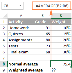
In mathematics and statistics, you calculate weighted average by multiplying each value in the set by its weight, then you add up the products and divide the products' sum by the sum of all weights.
In this example, in order to calculate the weighted average (overall grade), you multiply each grade by the corresponding percentage (converted to a decimal), add up the 5 products together, and divide that number by the sum of 5 weights:
((91*0.1)+(65*0.15)+(80*0.2)+(73*0.25)+(68*0.3)) / (0.1+0.15+0.2+0.25+0.3)=73.5
As you see, a normal average grade (75.4) and weighted average (73.5) are different values.
Calculating weighted average in Excel
In Microsoft Excel, weighted average is calculated using the same approach but with far less effort because Excel functions will do most of the work for you.
Calculating weighted average using SUM function
If you have basic knowledge of the Excel SUM function, the below formula will hardly require any explanation:
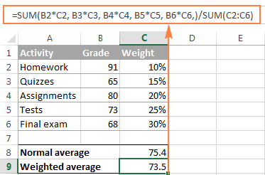
=SUM(B2*C2, B3*C3, B4*C4, B5*C5, B6*C6,)/SUM(C2:C6)
In essence, it performs the same calculation as described above, except that you supply cell references instead of numbers.
As you can see in the screenshot, the formula returns exactly the same result as the calculation we did a moment ago. Notice the difference between the normal average returned by the AVERAGE function (C8) and weighted average (C9).
Although the SUM formula is very straightforward and easy to understand, it is not a viable option if you have a large number of elements to average. In this case, you'd better utilize the SUMPRODUCT function as demonstrated in the next example.
Finding weighted average with SUMPRODUCT
Excel's SUMPRODUCT function fits perfectly for this task since it is designed to sum products, which is exactly what we need. So, instead of multiplying each value by its weight individually, you supply two arrays in the SUMPRODUCT formula (in this context, an array is a continuous range of cells), and then divide the result by the sum of weights:
Supposing that the values to average are in cells B2:B6 and weights in cells C2:C6, our Sumproduct Weighted Average formula takes the following shape:
=SUMPRODUCT(B2:B6, C2:C6) / SUM(C2:C6)
To see the actual values behind an array, select it in the formula bar and press the F9 key. The result will be similar to this:
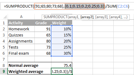
So, what the SUMPRODUCT function does is multiply the 1st value in array1 by the 1st value in array2 (91*0.1 in this example), then multiply the 2nd value in array1 by the 2nd value in array2 (65*0.15 in this example), and so on. When all of the multiplications are done, the function adds up the products and returns that sum.
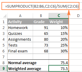
To make sure that the SUMPRODUCT function yields a correct result, compare it to the SUM formula from the previous example and you will see that the numbers are identical.
When using either the SUM or SUMPRODUCT function to find weight average in Excel, weights do not necessarily have to add up to 100%. Nor do they need to be expressed as percentages. For example, you can make up a priority / importance scale and assign a certain number of points to each item, as demonstrated in the following screenshot:
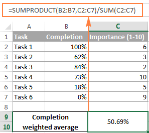
Well, that's all about calculating weighted average in Excel. You can download the sample spreadsheet below and try the formulas on your data. In the next tutorial, we are going to have a close look at calculating moving average. I thank you for reading and look forward to seeing you next week!
Practice workbook
Excel Weighted Average - examples (.xlsx file)
 by
by
47 comments
Your site provides an incredibly detailed and user-friendly guide on calculating weighted averages in Excel. The step-by-step instructions and clear examples make complex concepts easy to understand and apply. Thank you for such a valuable resource
What if your total grade is 33 and you get a 33/33? Can you use the same formula?
Please clarify your specific problem or provide additional details to highlight exactly what you need. As it's currently written, it's hard to tell exactly what you're asking.
Hi, I'm trying to calculate gender diversity for a country. When I look at overall gender diversity in a country overall, it shows 38% female population. However, when I split the data by functions or levels. The average would show me 58% female population, which is not correct. we would like to understand where each function is now, and how much they need to increase each year to reach these targets for their functions. If I split by functions and since the average is already showing 58% which is not correct, which formula should be used to accurately define? Please help.
Hi! Unfortunately, this information is not enough to recommend a formula to you. I don't know what data you are using, what formulas you are using and how you calculated 38% and 58%, how you split the data. If you give more information, I will try to help.
Calculating Estimation Average in Multiple Exams
Total exams count-10
But one student written only 8 exams reaming all present how to Calcuating Estimation Average in Excel
Plz let me what is the formula use above condition
I have bond trading data which consists of trade date, trade (buy/sell), bond issue, coupon, traded yield, traded clean price and traded dirty price. I keep adding the transactions as per those columns. I intend to compute the volume-weighted average (VWA) values per trade row. If it is a purchase (get VWA of the yield, clean and dirty for that bond issue). If it is a sale it looks up most recent VWA value for the respective bond issue and assigns/displays it.
More of a trading log with each row computing the VWA values per each entry - yield, clean and dirty. If purchase compute VWA values, if sale, lookup the last VWA values based on the bond issue (cannot sell something that is not there). This column data shall be used compute the profit and loss, per row (mainly upon sale, for purchases it is blank).
I am avoiding CSE array functions. Attempting to use SUMPRODUCT, but it breaks (generates wrong VWA
values) when there are more one purchase entries.
Hi!
I am not an expert in bond trading and therefore cannot guess what you want to calculate.
Explain what you want to calculate, and give an example of the source data and the expected result.
This Blog is helpful.
Hi,
Can u explain me this situation where I have an yearly data for every particular meal dish starting Jan-21 to Dec-21 on a daily level.
Now every dish is available for different no. of days in a week. For eg, Butter chicken will be available for all 7 days of a week but maybe the Turkey sandwich will be available only twice a week.
How do i calculate the daily weighted average for each dish.
Hello!
The formula for calculating the weighted average can be completely different depending on how your data looks. If column B is the quantity and column C is the price, then the formula might be:
=SUMPRODUCT(B2:B53, C2:C53) / SUM(C2:C53)
If this is not what you wanted, please describe the problem in more detail.
Thank you! This is very easy and helpful.
If given a chance to use calculator and Microsoft excel, which one will you choose?
Hi - how does one calculate a weighted average if you only have one data set without a weight column. For instance, I have 6 figures (5 of them are under $102 and one is $1M). The simple average here would be skewed by the $1M. So how would I obtain a more "weighted" average here?
This is the sample data:
$101,
$102,
$91,
$100,
$90,
$1,000,000
Hello!
For non-typical values, it is recommended to calculate not the average, but the median. You can learn more about mean, median and mode in this article.
I hope it’ll be helpful.
Hi,
No need to divide by the percentage as it is always like dividing by 1.
SUMPRODUCT(values_range, weights_range) is enough.
That's correct your weights should add to 1 so no need to divide by 1. I mean you can but there's no point.
Don't think so - you don't get the same result
Op Or
666.29 -10.79
734.57 9.45
800.39 41.7
2201.25 40.36
Weighted Average=?
HELP!!!!
How do I calculate the weighted average?
Month= 1-12
Amount= 159K; 67K; 92K; 83K; 125K; 119K; 213K; 85K; 79K; 113K; 124K; 183K
Hello Lynn!
I hope you have studied the recommendations in the above tutorial. Please let me know in more detail what formula you used and what problem or error occurred. In that case I will try to help you.
I will be holding a random drawing for 80 people. Each person will have a number of raffle tickets earned before the drawing. I'd like to assign a weight to the people who have more raffle tickets than people who have less. Example: Person A has 10 raffle tickets and Person B has 3 raffle tickets, I'd like to assign a specific percentage for Person A and Person B. Person A probability should be higher than Person B. Is there a way I can do this and then hold a random drawing?
if
Cutoff = 60 Marks
Max Score = 70 Marks
Weightage = 20%
how to calculate score ( Weightage) if any body have 65 Marks
Thank you, I found the tutorial very useful!
I want to perform all the calculations in one cel,item,Quantity and Moisture weighted average in exal
How do I get the weighted aver per FY (total?
FY16 FY17 FY18
$4,600 $3,618 $53
($58) ($9) ($460)
$140 $463 $99
$6,627 $6,101 $6,420
$0 $0 ($694)
($8) ($2,303) $0
($4,501) ($6,079) ($1,902)
$6,800 $1,791 $3,516
How would i add a new number to a cell and give me an average of the amount of entries
first entry 46
a week later i want to add 52 to the same cell
a week later i want to add 58 to the same cell
I want the results to be 52 printed in the cell
156 / 3 = 52
Hello, Gerald.
If you want to perform all the calculations in one cell, you'll have to manually update its content each time. If, however, your task if to find average value of multiple cells, please have a look at the following article on our blog:
How to calculate average (mean) in Excel - AVERAGE, AVERAGEIF, AVERAGEIFS formula examples
Hope you'll find this information helpful.
So a bit more complex of a weighing that I need and I have struggled with it for a while.
I basically have two separated weighted categories which each have 3 internal weighted categories but everything combines for one single score. I could not get the sum product function to align with the answer that populates from our automatic dashboard system .
Example:
Total percentage of score is 100% broken into two main categories at 70 and 30 percent
Category 1: 70% weight
Sub Category 1 weight: 40% of the total 70%
Sub Category 2 weight: 35% of the total 70%
Sub Category 3 weight: 25% of the total 70%
Category 2: 30% weight
Sub Category 1: 33.3% of the total 30%
Sub Category 2: 33.3% of the total 30%
Sub Category 3: 33.3% of the total 30%