Now, that we've learnt how to enter dates and time to your spreadsheet, it's time to talk about the ways of calculating time in Google Sheets. We'll discuss the ways of finding time difference in detail, see how to sum dates and time together, and learn to display only date or time units and set them apart completely.
How to calculate time difference in Google Sheets
When you're working on some projects, it is usually important to control how much time you spend. This is called elapsed time. Google Sheets can help you calculate the time difference in a lot of various ways.
Example 1. Subtract time to get the time duration in Google Sheets
If you have your start time and end time, it's not a problem to find out the time spent:
Let's assume the start time is in column A and the end time is in column B. With a simple subtraction formula in C2, you will find how much time this or that task took:
=B2-A2
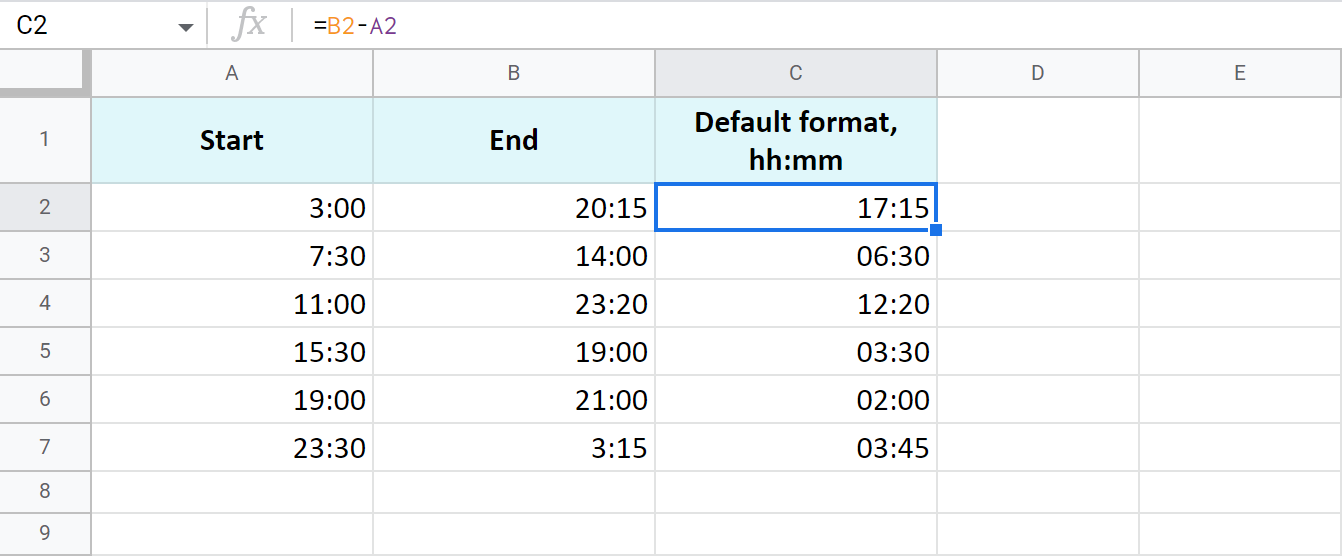
The time is formatted as "hh:mm" by default.
To get the results as hours only or as hours, minutes, and seconds, you need to apply a custom format with the corresponding time codes: h and hh:mm:ss. Google even offers a special number format for cases like this - Duration:
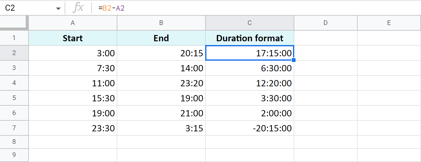
Tip. To apply the custom time format, go to Format > Number > Custom number format in your spreadsheet menu.
Example 2. Calculate time duration in Google Sheets using the TEXT function
Another trick to calculate the time duration in Google Sheets involves the TEXT function:
=TEXT(B2-A2,"h") - for hours
=TEXT(B2-A2,"h:mm") - for hours and minutes
=TEXT(B2-A2,"h:mm:ss") - for hours, minutes, and seconds
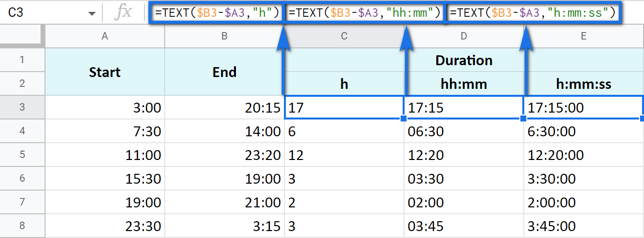
Note. See how the records are aligned to the left? Because the TEXT function always returns the results formatted as a text. This means these values cannot be used for further calculations.
Example 3. Time difference in hours, minutes, and seconds
You can track the time spent and get the result in one time unit disregarding other units. For example, count the number of only hours, only minutes, or only seconds.
Note. To ensure correct results, your cells should be formatted either as numbers or automatically: Format > Number > Number or Format > Number > Automatic.
-
To get the number of hours spent, subtract your start time from the end time and multiply the result by 24 (since there are 24 hours in one day):
=(End time - Start time) * 24You will get a time difference as a decimal:

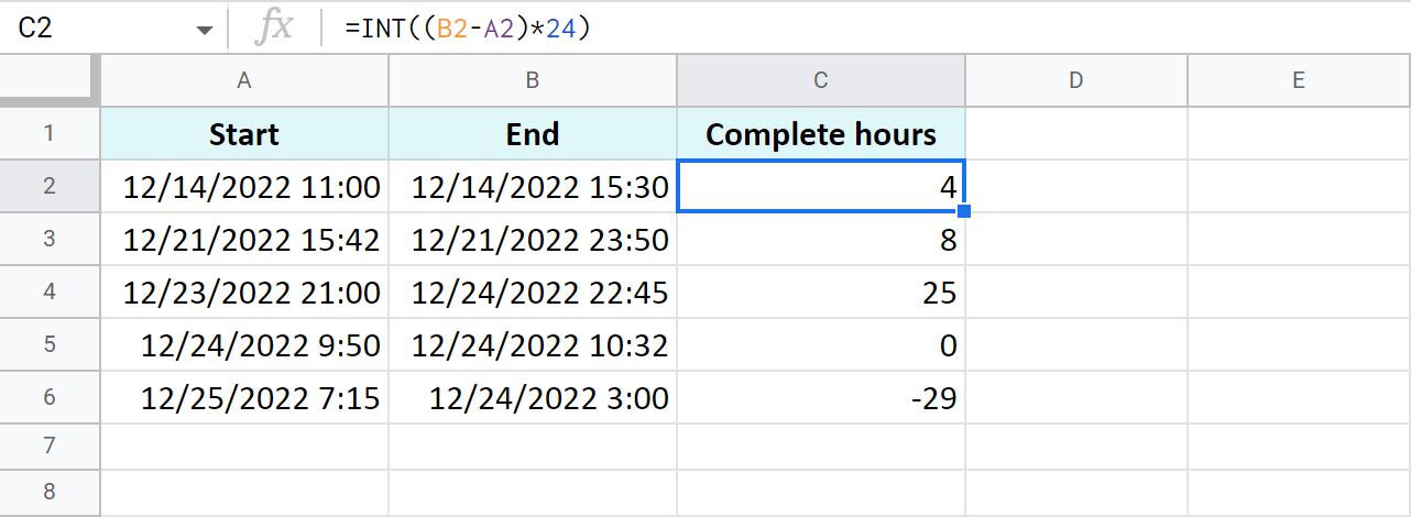
If the start time is greater than the end time, the formula will return a negative number, like in C5 in my example.
Tip. The INT function will let you see the number of complete hours spent since it rounds numbers down to the nearest integer:
-
To count minutes, subtract the start time from the end time and multiply whatever you get by 1,440 (since there are 1,440 minutes in one day):
=(End time - Start time) * 1440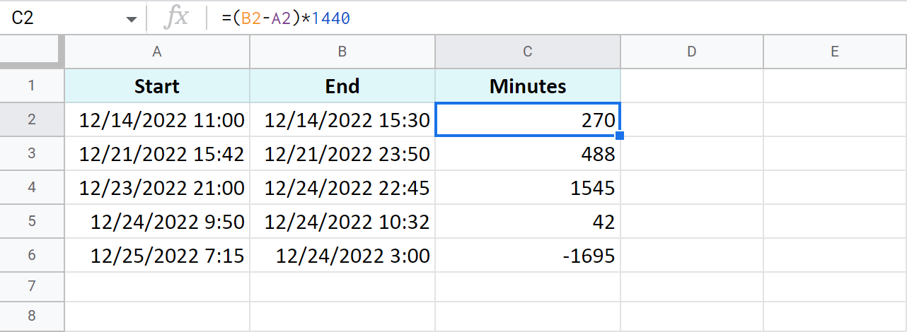
-
To find out how many seconds passed between two times, the drill is the same: subtract the start time from the end time and multiply the result by 86,400 (the number of seconds in a day):
=(End time - Start time) * 86400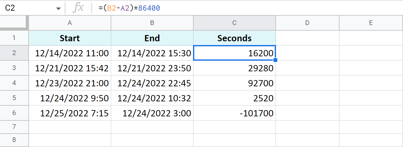
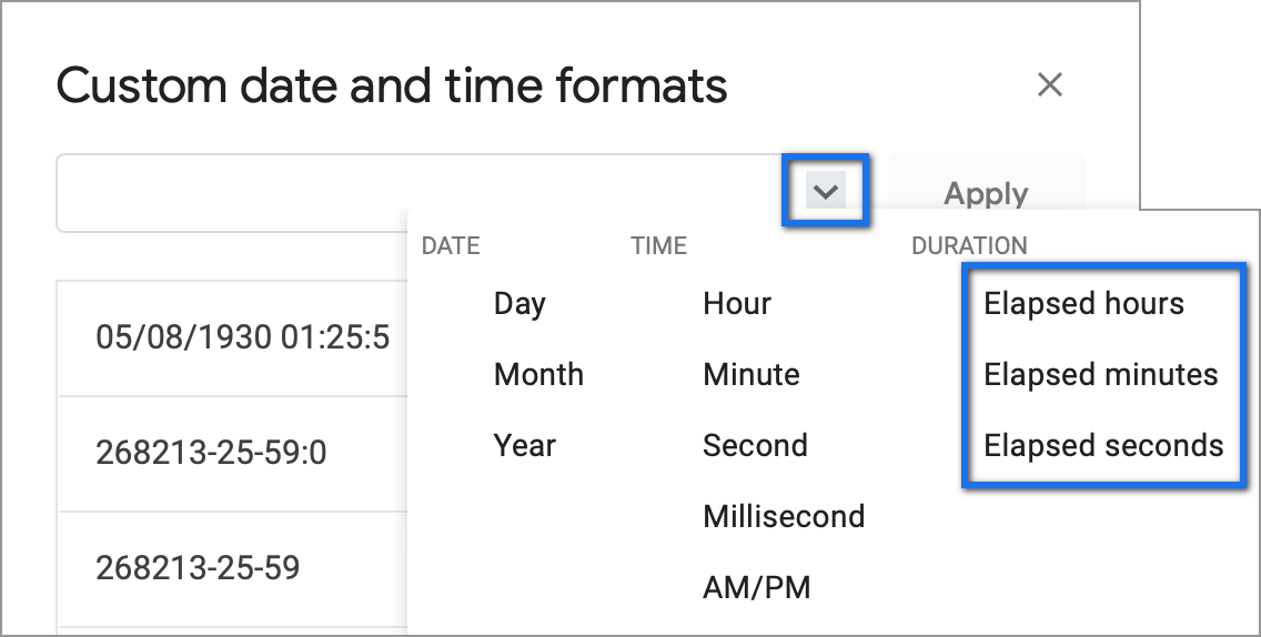
Tip. You can avoid multiplying in all these cases. Just subtract times first, and then apply elapsed time format from Format > Number > Custom date and time. If you click the down arrow to the right of the text field, you'll be able to choose between additional date and time units:
Example 4. Functions to get the time difference in a Google spreadsheet
As always, Google Sheets equips you with three particularly useful functions for this purpose.
Note. These functions work only within 24 hours and 60 minutes and seconds. If the time difference exceeds these limits, the formulas will return errors.
=HOUR(B2-A2)- to return hours only (without minutes and seconds)=MINUTE(B2-A2)- to return minutes only (without hours and seconds)=SECOND(B2-A2)- to return seconds only (without hours and minutes)

How to add and subtract time in Google Sheets: hours, minutes, or seconds
These operations can also be achieved with two techniques: one involves basic math calculations, another - functions. While the first way always works, the second one with functions works only when you add or subtract units less than 24 hours, or 60 minutes, or 60 seconds.
Add or subtract hours in Google Sheets
-
Add less than 24 hours:
=Start time + TIME(N hours, 0, 0)Here's how the formula looks on real data:
=A2+TIME(3,0,0)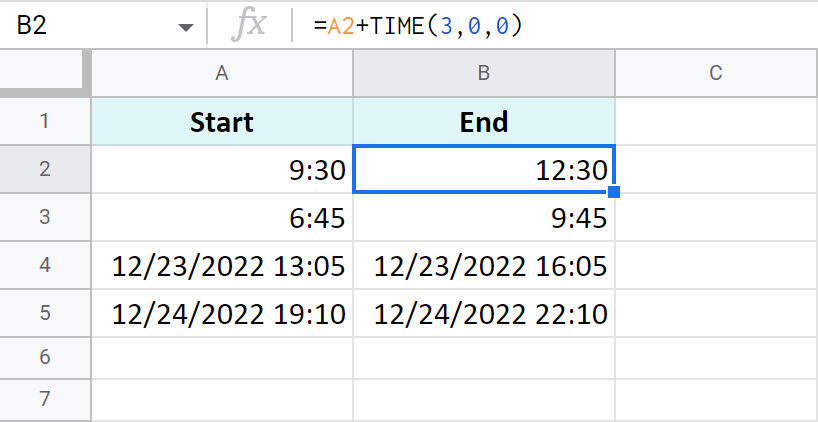
-
Add more than 24 hours:
=Start time + (N hours / 24)To add 27 hours to the time in A2, I use this formula:
=A2+(27/24)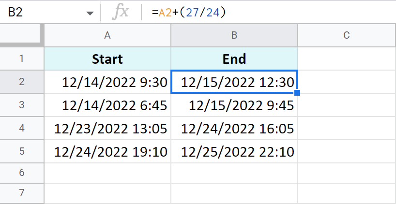
- To subtract 24 and more hours, use the formulas above as a basis but change the plus sign (+) to the minus sign (-). Here's what I've got:
=A2-TIME(3,0,0)- to subtract 3 hours=A2-(27/24)- to subtract 27 hours
Add or subtract minutes in Google Sheets
The principle of manipulating minutes is the same as with the hours.
-
There's the TIME function that adds and subtracts up to 60 minutes:
=Start time + TIME(0, N minutes, 0)If you are to add 40 minutes, you can do it like this:
=A2+TIME(0,40,0)If you are to subtract 20 minutes, here's the formula to use:
=A2-TIME(0,40,0)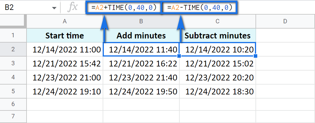
-
And there's a formula based on simple arithmetic to add and subtract over 60 minutes:
=Start time + (N minutes / 1440)Thus, here's how you add 120 minutes:
=A2+(120/1440)Put the minus instead of plus to subtract 120 minutes:
=A2-(120/1440)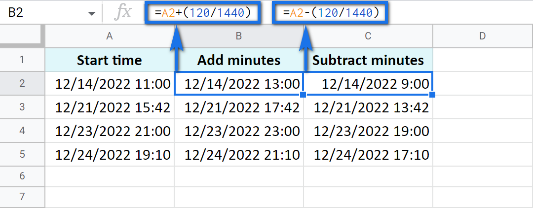
Add or subtract seconds in Google Sheets
Seconds in Google Sheets are calculated in the same manner as hours and minutes.
-
You can use the TIME function to add or subtract up to 60 seconds:
=Start time + TIME(0, 0, N seconds)For example, add 30 seconds:
=A2+TIME(0,0,30)Or subtract 30 seconds:
=A2-TIME(0,0,30) -
To calculate over 60 seconds, use simple maths:
=Start time + (N seconds / 86400)Add 700 seconds:
=A2+(700/86400)Or subtract 700 seconds:
=A2-(700/86400)
How to sum time in Google Sheets
To find the total time in your table in Google Sheets, you can use the SUM function. The trick here is to choose the correct format to display the result.
By default, the result will be formatted as Duration - hh:mm:ss
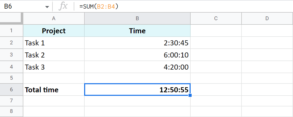
But most often the default time or duration format won't be enough, and you will need to come up with your own one.
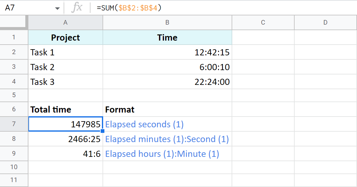
A7:A9 cells contain the same time value. They are just displayed differently. And you can actually perform calculations with them: subtract, sum, convert to decimal, etc.
Extract date and time from a full "date-time" record
Let's imagine that one cell in Google Sheets contains both, date and time. You want to set them apart: extract only the date to one cell and only time to another.
Split Date time using Number format
In order to display date or time in one cell on your screen or to print it, just select the original cell, go to Format > Number and choose Date or Time.
However, if you'd like to use these values for future calculations (subtract, sum, etc.), this won't be enough. If you don't see the time unit in a cell, it doesn't necessarily mean that it's absent, and vice versa.
So what do you do?
Split Date time using formulas
Google stores dates and time as numbers. For example, it sees the date 8/24/2017 11:40:03 as the number 42971,4861458. The integer part represents the date, the fractional - time. So, your task is down to separating integer from fractional.
- To extract date (integer part), use the ROUNDDOWN function in cell B2:
=ROUNDDOWN(A2,0)
The formula rounds the value down and casts the fractional part away.
-
To extract time, place the following subtraction formula into C2:
=A2-B2 -
Copy the results into the third row and apply Date format to B3 and Time format to C3:

Use the Split Date & Time add-on
You may be surprised but there's one special add-on for this job. It's really small and easy but its contribution to Google Sheets cannot be overstated.
Split Date & Time splits all Date time records in your entire column at once. You control the desired outcome with just 4 simple settings:
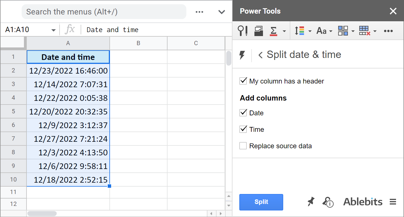
You tell the add-on:
- Whether there's a header row.
- If you want to get the Date unit.
- If you want to get the Time unit.
- And if you'd like to replace your original column with the new data.
It literally takes the burden of splitting date and time units off your shoulders:
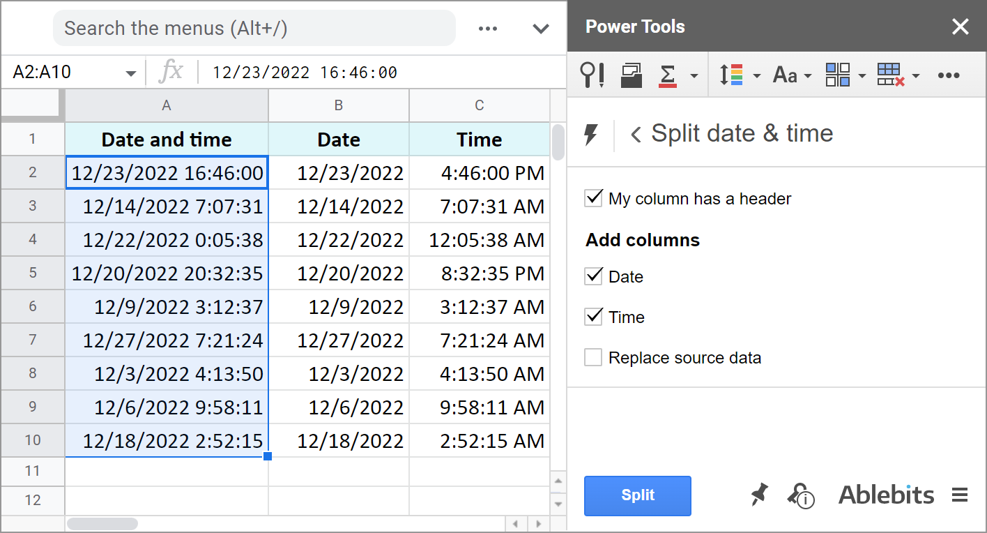
Split Date & Time is part of the Power Tools collection so you will have more than 40 other useful tools for Google Sheets at hand.
These are the ways to not only display date or time, but to separate them to different cells. And you can perform various calculations with these records now.
I hope these examples will help you solve your tasks when working with dates and time in Google Sheets.
Spreadsheet with formula examples
Calculating time in Google Sheets (make yourself a copy to practice)
 by
by
393 comments
Hi!
I have a sheet with multiple cells where time is entered in [hh]:mm format. I have another cell finding the sum of all of those time cells. It calculates and displays the time correctly unless it is 60:00 or greater. How can I format this sum to allow for more than 60 hours?
Thank you!
Hi Kristy,
For me to be able to help you, please specify a couple of time units as you have them in cells, the exact formula you're using to sum them, and the format you applied to the resulting cell.
Hi Natallia, hope all is well with you.
Can you help me in understanding time and duration display?
1. When I enters 24:00 to cell then it display as 00:00 and calculate duration as expected. But in formula/value row displays as "31.12.1899 00:00:00"
2. I collect duration of 2 tasks then SUM it. This SUM never can be grate then 24:00 due I calculate durations for 1 day. When SUM < 24:00 then it displays correctly: 22:00, 23:30, etc. But 24:00 shows as 00:00. How can i tell true 00:00 from trimmed 24:00?
Thank you!
Hi Anatolii,
Thank you for responce!
For example:
Task1 duration=SUM(B2-A2;D2-C2;...) or your ARRAYFORMULA(SUM(TIME(HOUR({...
Task2 duration=SUM(C3-B3;E3-D3;...) or your ARRAYFORMULA(SUM(TIME(HOUR({...
Task duration calculates as expected, no questions
Sum of Task1 and Task2 = Task1 duration + Task2 duration
(Time without Task1 and Task2) = 1-(Sum of Task1 and Task2)
Task1 duration | Task2 duration | Sum of Task1 and Task2 | Time without Task1 and Task2
14:30 | 09:00 | 23:30 | 00:30 | as expected
13:00 | 09:00 | 22:00 | 02:00 | as expected
16:00 | 08:00 | 00:00 | 00:00 | ???
14:00 | 10:00 | 00:00 | 00:00 | ???
2 last rows expected as
16:00 | 08:00 | 24:00 | 00:00 |
14:00 | 10:00 | 24:00 | 00:00 |
or 1 day without 24:00 but this can`t be used in calculations
Thank you!
Thank you for the samples, Anatolii.
As I already mentioned, 24:00 as a time is 00:00 for Google Sheets by default. There's nothing you can do with that.
In your case, I'd advise changing the number format from Time to Duration. You will then see 24:00:00 in your cells and that's exactly what you need. If you don't want to see seconds, after applying the Duration format go to Format > Number > Custom date and time, and remove Elapsed seconds from the format.
For some reason I do not see my reply :(
Please look at the sample data and results
Thank you!
Thank you for help!!! A very valuable note about the empty cell. It help me a lot!
I also used the formula =HOUR(Duration) to check the correctness of the duration. Even when the duration looks correct, this formula throws an error when there is a negative number.
The final solution at the sheet with the some name
Once again, thank you very much for your help! :))
You're most welcome, Anatolii!
Thank you for sharing your file, Anatolii. I duplicated your sheet within your file and entered correct formulas based on the description in the file, please have a look.
Your formulas won't do because each empty cell is treated as 24 hours resulting in negative numbers. Hence, my formulas with TIME, HOUR, MINUTE are the ones to work with. They didn't work for you at first because you needed to switch the TIMES functions places. When you compare my formulas from new sheet with the formulas you used on your sheet, you'll see what I mean.
Hope this helps :)
Hi Natalia! Thanks for your help, but I'm at a dead end.
Custom date and time format resulted in unexpected data, I got negative numbers after summing the durations! How can it be?
I have shared a sample table with data and results. Can you take a look please?
yellow cells show incorrect data
Thank you!
Hello,
I am trying to keep track of "Door(arrival time) to Activation time" in minutes. Sometimes the activation time is minutes before the arrival/Door time. When this happens, I receive a negative number (obviously). What is the formula to achieve the difference between the two times? And then when I receive this negative number, is there a way to have it read as "0"?
I currently have the Page time, the Arrival Time and my "Door to Activation time" columns in the TIME Format so when I attempt the simple =J37-H37 formula I receive results in a decimal. I need the decimals to populate as whole numbers and I need the negative result to populate as "0".
For instance, EMS crew pages the ER to notify them of an incoming patient at 07:50 AM. The patient arrives to the ER at 08:00 AM. What I am trying to calculate is the page(activation) time 07:50 AM minus the Arrival time 08:00 AM = - 0.01. I need this decimal to result as a whole "0".
Alternatively, 08:00 AM - 07:50 AM= 0.01. I need this to translate to 10 (minutes)
Any and all help will be greatly appreciated! My brain hurt even typing this out.
Hello Holland,
For 0.01 to appear as 10 minutes, make sure to format the resulting cell as Duration or one of the custom formats as shown in this part of the article.
For -0.01 to appear as 0, you need to incorporate IF function to your calculations.
Currently i am working on the time calculation of task completed tasks only which was accepted first and then check out later on after completion. both of them are in DD-MM-YY HH:MM formats. The list contains both the completed task with check out date and time stamp and pending with no any values.
now i am making a dashboard so that i need to see how many task is completed in the time gap of 1 hour from 7 am to 7 pm . here i need to count of completed task in each time frame with for day wise filtration.
similarly i need the number of total schedule task and total assigned task in the same ways , thats why split formula wont be beneficial for me. can you help me out.
Please mail me if you need sample of dump file.
Hello Bishwas,
I'm sorry but your task is not clear. For me to be able to help you, please share a small sample spreadsheet with us (support@apps4gs.com) with 2 sheets: (1) a copy of your source data (2) the result you expect to get. The result sheet is of great importance as it gives us a better understanding than any text description.
I kindly ask you to shorten the tables to 10-20 rows.
Note. We keep that Google account for file sharing only and don't monitor its Inbox. Do not email there. Once you share the file, just confirm by replying to this comment.
I'll look into it and try to help.
Hi Natalia,
I have added different tasks in one column of google sheets and each one of them has "Start" and "End" time written in different columns. I also have added another column for calculation of the total dedicated hours to each of the tasks with this formula: = TEXT($E2 - $D2,"hh:mm") considering that Start is in D2 and End is in E2. Now I want to sum ALL of the dedicated hours for all of the tasks and see how much I had spent on all of the tasks at the end of the day. I cannot add a formula for that. Can u pls help?
Are You trying to add text strings?
Thar will not give you a time value !
Hi Niels
Here is more info:
Column B: Dedicated Hours Per Day - Predicted Column --> No formula in the rows. Here I have only added predicted hours in hh:mm:ss format:
00:10:00
02:00:00
01:30:00
00:30:00
Column C: Dedicated Hours Per Day - Actual Column --> = TEXT($E2 - $D2,"hh:mm")
00:10
Column E: End
Column D: Start
The data here in these two columns have been written the same as the first column. Only hh:mm:ss manually.
I just wanted to provide more info. I need the SUM of column C so that I can prepare it with the SUM of column B which I could have with no problem. What should be changed here? Any suggestions for me?
Hi Naqme,
What Niels means is that you're using the TEXT function to get the duration. The TEXT function returns values as text (even though you see it as if time units) and Google Sheets doesn't tally text values. I mentioned this limit at the end of this section regarding the TEXT function.
To be able to sum times, use this method instead. It also mentions how to apply the custom time format so the result looks as needed.
Excellent explanations, thank you for you time. I am using a time tracker on my iphone (ATracker) for tracking client times for 3 different categories (tags) and it shows say 4:38 and I want to convert this to minutes. E.g. 01:30 should be 90 mins, however, I can't get it to convert with anything I tried. Could you give me a formula just to convert the hours:minutes into only minutes. Greatly appreciated, Steve.
P.S. I have tried this formula and got the closest =INT(C12)*60*60+(C12-INT(C12))*24*60 and this gives me seconds and I divided the seconds by 60. When there is only hours, it works! But when I put minutes to it, it doesn't. 1.5 hours = 67.2 minutes
Hi Stephen,
How exactly do your values look in cells? Hours:minutes (1:30) or as intigers (1.5)?
1. 2. 3
4 = 14400 =240
1.30 = 4032 =67.2
The formula in 2 (14400) is [fx = INT (C12) *60*60+(C12-INT (C12))*24×60] C12 in this formula represents the 1 column
The formula in 3 (240) is = [=E12/60] E12 represents the 2 column
Not sure if this is what you asked for?
Hopefully this stays formatted.
Thank you for the clarification, Steve.
Try this formula:
=INT(C12)*60 + (C12-INT(C12))*100
It correctly converts 4 and 1.30 hours to 240 and 90 minutes correspondingly on my side.
Hi Natalia,
Thank you for your help to everyone!
First, sorry for my English. I need help with a formula. =goal-time. I would like to get the sustract between 2 cells. One is the goal: 1h (01:00:00,000), and the other the amount of time worked (e.g. (00:48:00,000). Then it will show the remained time. But when the times is higher that the goal, it doesn't work. I would like to show how much time remained or how much time I worked above the goal.
=01:00:00,000-00:48:00,000 --> =00:12:00,000
But when for e.g. is 72 minuts =01:00:00,000-00:62:00,000 --> the result is something like 23:58:00,000.
Can you help me? Thank you.
Hello Stef,
Your second example works fine on my side. First of all, Google Sheet converts 00:62:00.000 to 01:02:00.000, because that's how Duration looks. Then it subtracts it from 01:00:00.000 and I'm getting -00:02:00.000 as a result.
Please double check your values and cell format (Format > Number > Duration). And the formula you're using, of course. It's better to enter values in cells and then use a formula like =A2-B2 so Google understands your values.
Yes... cell format... Thanks so much!
You're most welcome, Stef 😉
How to add (subtract) hours in format "1.5"?
For example A1 = "23:00" A2 = "1.5" A3 (formula?) = "00:30"
Hello Paul,
Try this formula:
=TEXT(A1+A2/24,"hh:mm")
how to add current time in google sheet
Hello vignesh,
You will learn it in this article: Google Sheets date and time functions
I have a challenge subtracting time where the end time is midnight. How do I format the cell for midnight?
Find attached a link to the sample spreadsheet: https://docs.google.com/spreadsheets/d/1Q0pxFwYAzd8AtRGlQQMkvj8wlH9kgn9uRP_jMlKTcrI/edit?usp=sharing
Thank you for your help.
Hello Yohanna,
I'm afraid you'll have to add dates to the time units (in rows with 0:00 in cells) so Google Sheets understands there are dates implied and calculates everything correctly.
Hi Natallia,
Hope all is well with you.
I would appreciate your help. Need a formula for:
Program starts a 9 (let's say B1) arrival time can be either before 9 (let's say 8:49- C1) the arrival could be on time or after the start time. If the arrival is before the start time, there will be a $10 charge for every 15 minutes, and $1 per minute after one hour. There is a 10 minutes grace period. No charges if it is on time or after. Hope my explanation make sence
Thank you in advance for your help.
Hi Emma,
For me to be able to help you better, please share a small sample spreadsheet with us (support@apps4gs.com) with 2 sheets: (1) a copy of your source data (2) the result you expect to get. The result sheet is of great importance as it gives us a better understanding than any text description.
I kindly ask you to shorten the tables to 10-20 rows.
Note. We keep that Google account for file sharing only and don't monitor its Inbox. Do not email there. Once you share the file, just confirm by replying to this comment.
I'll look into it and try to help. Thank you.
Hello!
I'm using sheets to help track the pay for our nanny we share with another family. I need help figuring out shared time. Our nanny gets paid $25/hr, but when it's both kids together, the families split the bill to pay $12.50/hr each. Some days are just one kid, so that family just pays $25/hr for the whole day. Some days are one kid in the morning, the second kid comes for a few hours in the afternoon, and then the last few hours with just the first kid. So one family pays the morning as $25/hr, the shared time as $12.50, and the last hours as $25/hr; the second family pays just $12.50/hr for the shared time. Both kiddos do this pattern, so either one might have more time in than the other (meaning a superset as a default assumption didn't work.)
How do I ask sheets to find the amount of time the two kids shared? I can have separate "time in" and "time out" columns for each kid, but setting a formula to calculate the overlapping hours has been so tricky that we've just been doing it by hand!
Appreciate the help!
Rose
Hello Rose,
I'm sorry it's hard to provide any formula because I have no idea how your data is arranged. For me to be able to help you, please share a small sample spreadsheet with me (support@apps4gs.com) with 2 sheets: (1) a copy of your source data (2) the result you expect to get. The result sheet is of great importance as it gives a better understanding than any text description.
I also kindly ask you to shorten the tables to 10-20 rows.
Note. We keep that Google account for file sharing only and don't monitor its Inbox. Do not email there. Once you share the file, just confirm by replying to this comment.
I'll look into your task and try to help.
Hi Natalia, hope you're doing well!!
I have a cell with a data just like 18/08/2023 11:12:00 (Cell FM3) and another cell with the numer of working hours = 48 (Cell FN3). In another sheet i have a list with the holidays troughout the year, and i consider 08h and 30 minutos as working hours per day.
Is there any how to calculate de date + 48 working hours, considering 8h and 30 minutes per day? I've tried everything but i couldn't get by....
Thanks!!
Hi John,
Can you please specify what result exactly you want to achieve? What should the formula show as a result?
Hello, Natalia! Sorry if I couldn't be clear enough. I would like a formula for Google Sheets that adds 48 working hours to the FM3 cell that contains "18/08/2023 11:12:00". For example, if we consider 48 running hours, the formula would return "20/08/2023 11:12:00", but I would like to specify working hours, where working hours for me are from 08:00 to 12:00, and from 1:30 pm until 6:00 pm. (12:00 - 13:00pm lunch time). In other words, the total number of working hours per day, from 8:00 am to 6 pm, is 8:30 (8h 30min). I've done a lot of research, but you're the only person on the entire internet who seems to be able to accomplish this formula! Thanks for replying!
Thank you for additional explanation, John! Could you please share a sample table with me (support@apps4gs.com)? Understanding how your data is arranged will help me find the most suitable solution for you.
Note. We keep that Google account for file sharing only and don't monitor its Inbox. Do not email there. Once you share the file, just confirm by replying to this comment. Thank you.
Just sent! Thank you very much for your support!!!
Hi John,
I'm sorry I don't see any file shared from you. To grant me access to your data, press the Share button at the upper right corner of Google Sheets and enter support@apps4gs.com to share the file directly. Thank you.
Hi just want to ask what to do here because I have tried the formula for the other cells but it wont get the total number of hours. for example a total number of worked hours in one month is 240 hours, I have input 12 hours each day, for example I put 12 hours for 5 days and one day for 9 hours, and when you total it it will show negative sum. together with other. but the other cells are accurate
Hi claire,
In what format do you enter those hours? How is your cell with the resulting formula formatted? What formula exactly are you trying to use?
Hello, I am wanting to create a time sheet for some fellow employees but I cannot find a formula that shows how to get the total hours worked from doing the clock in, out, in, out for their lunch breaks (example: in 6:45 am, out 1:20 pm, in 2:05 pm, out 5:20 pm = 9 hours and 50 minutes worked) I cannot get it to equal the time total worked with any formula I have tried. Please let me know if there is a way to do that.
Hello samantha,
Just calculate the time difference between the start time and end time as shown in this part of the article and then subtract the lunch:
=D2-A2-(C2-B2)
Hi there,
I'm trying to efficiently figure out my employees hours worked and pay for those hours. So I have figured out how to subtract time started from time ended and then how do I translate that time- back to hours so I can multiply that by their hourly pay. For example:
Employee 1: Clock In- 16:15 Clock Out- 21:30 and get 5:15 then I try to multiply this number by $18/hr and am getting a wacky number. any advice??
Hi Beth,
Try to multiply your time difference by 24 to get the result as a decimal first. Then it will multiply by an hourly rate correctly. Please see this section for formula examples: Time difference in hours, minutes, and seconds
Natalia, firstly you are a wizard when it comes to this! Thanks for your help in advance!
Here's the layout of my timesheet (that gets fed from the form)
Timestamp Name Email Your Position Date Completed Time Started Time Completed Hours worked
2/6/2024 17:06:06 sample sample 2/5/2024 3:45:00 PM 5:00:00 PM 1.15
I'm trying to have the sheet calculate the hours worked working with the AM PM time - is that possible?
Appreciate your lovely words, Avi!
For your task, you need to subtract time started from time completed (and multiply it by 24 if you'd like to get the result as a decimal). See this section for formulas examples: Time difference in hours, minutes, and seconds
Hi Natalia, I am building a google sheets that allow me to arrange schedule for employees.
After we key in time in and time out, I already make it to be able to auto calculation for us to count the total working hours. But besides that, I need your help on this:
If the working hours is more than 7.5hours, need to minus one hour break time.
If the working hours is less than 7.5hours, no need to minus any break time.
How do I do that? Kindly assist.
Thank you so much.
Hello KY,
The IF function will help you check if the working hours are more/less than 7.5 hours and add or subtract the required amount of time correspondingly.
Hi There,
I am building a sheet that will allow me to calculate a "premium" on an employees hourly rate based on the time of day. For example, depending on the time of day, the employee may make an additional 10% or 20% premium. The goal of the grid I am building, is to allow a user to enter someone's start time, have the remaining hours auto populate (using the time function to add an hour to each previous hour) and then use an IF AND function to check whether each hour is within a certain "premium" window and then apply said premium to their hourly.
I am using the following formula to auto populate the hours, adding one hour to the previous hour: =B5+TIMEVALUE("01:00:00") Note: I have also used the TIME function interchangeably to no avail.
I am using the following formula to evaluate the hour and determine which premium, if any, to apply to the hourly rate: =IF(AND($B6=TIMEVALUE("07:00:00")),$B$3*1,IF(AND($B6>=TIMEVALUE("20:00:00"),$B6=TIMEVALUE("00:00:00"),$B6<TIMEVALUE("07:00:00")),$B$3*1.2,"FALSE")))
Unfortunately, when the hours cross over from prior to midnight to after midnight (i.e. 11pm to 1am), the time evaluation formula does not detect any of the hours as falling between the 12:00am to 7:00am window, which should apply a 20% premium.
Any idea's how to adjust either formula to allow for this?
Hi Zach,
For me to be able to help you better, please share a small sample spreadsheet with us (support@apps4gs.com) with 2 sheets: (1) a copy of your source data with your formula (2) the result you expect to get. I kindly ask you to shorten the tables to 10-20 rows.
Note. We keep that Google account for file sharing only and don't monitor its Inbox. Do not email there. Once you share the file, just confirm by replying to this comment.
I'll look into your task and try to help.
Thanks Natalia! I have shared a sample sheet.
Thank you for creating a sample, Zach!
I entered another formula that works in the copy of the sheet, please take a look:
=IF(AND(HOUR($B5)<20,HOUR($B5)>=7),$B$3*1,IF(AND(HOUR($B5)>=20,HOUR($B5)<=23),$B$3*1.1,IF(AND(HOUR($B5)>=0,HOUR($B5)<7),$B$3*1.2,"FALSE")))
It looks like TIMEVALUE still accounts for dates (though its stated in its Help that dates are ignored) because your formula works as soon as I clear B5 and no time units seem to fall to "another day" (with 00:00) anymore. Anyways, the HOUR function solves this problem.
Thank you so much Natalia! You are THE BEST!
My pleasure, Zach! 😊
Hi Natalia
I'm trying to get the duration of 2 cells showing an event's start time and end time, but I want the format to be in days, hours, and minutes. for example the duration should be displayed as follows: 2 days 4 hours 34 minutes. What formula can I use?
Hi Rose,
Please try this formula:
=IF(B2>A2,CONCATENATE(DATEDIF(A2,B2,"D")&" days ",TEXT(MOD(B2-A2,1),"hh")," hours ",TEXT(MOD(B2-A2,1/24),"mm")," minutes"),"")
I have tried to use the formula you gave above, however, the formula keeps giving me 12 minutes for all the differences in time. I've tried to copy the example below so you can understand.
17/01/2024 12:20 18/01/2024 08:11 1 days 19 hours 12 minutes
18/01/2024 09:34 18/01/2024 10:49 0 days 01 hours 12 minutes
18/01/2024 11:24 18/01/2024 11:29 0 days 00 hours 12 minutes
18/01/2024 11:42 18/01/2024 12:04 0 days 00 hours 12 minutes
18/01/2024 12:06 18/01/2024 13:59 0 days 01 hours 12 minutes
18/01/2024 11:59 18/01/2024 14:01 0 days 02 hours 12 minutes
18/01/2024 14:35 18/01/2024 14:39 0 days 00 hours 12 minutes
18/01/2024 16:36 18/01/2024 16:38 0 days 00 hours 12 minutes
18/01/2024 00:06 19/01/2024 09:07 1 days 09 hours 12 minutes
for the example above, I used the formula below. I'm not sure if I'm writing it wrongly or otherwise. Please kindly advise
=IF(H60>G60,CONCATENATE(DATEDIF(G60,H60,"D")&" days ",TEXT(MOD(H60-G60,1),"hh")," hours ",TEXT(MOD(H4-G4,1/24),"mm")," minutes"),"")
Hi Rose,
Thank you for providing the sample. Try this formula instead:
=INT(H60-G60) & " days " & HOUR(H60-G60) & " hours " & MINUTE(H60-G60) & " minutes"
This worked perfectly. thanks a lot Natalia
You're most welcome, Rose!