In this tutorial, we will look at how to align cells in Excel as well as how to change text orientation, justify and distribute text horizontally or vertically, align a column of numbers by decimal point or specific character.
By default, Microsoft Excel aligns numbers to the bottom-right of cells and text to the bottom-left. However, you can easily change the default alignment by using the ribbon, keyboard shortcuts, Format Cells dialog or by setting your own custom number format.
How to change alignment in Excel using the ribbon
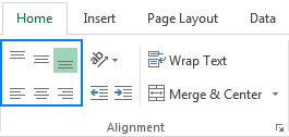
To change text alignment in Excel, select the cell(s) you want to realign, go to the Home tab > Alignment group, and choose the desired option:

Vertical alignment
If you'd like to align data vertically, click one of the following icons:
- Top Align
 - aligns the contents to the top of the cell.
 - Middle Align
 - centers the contents between the top and bottom of the cell.
 - Bottom Align
 - aligns the contents to the bottom of the cell (the default one).
Please note that changing vertical alignment does not have any visual effect unless you increase the row height.
Horizontal alignment
To align your data horizontally, Microsoft Excel provides these options:
- Align Left
 - aligns the contents along the left edge of the cell.
 - Center
 - puts the contents in the middle of the cell.
 - Align Right
 - aligns the contents along the right edge of the cell.
By combining different vertical and horizontal alignments, you can arrange the cell contents in different ways, for example:
Align to upper-left |
Align to bottom-right |
Center in the middle
|
 |
 |
 |
Change text orientation (rotate text)
Click the Orientation button on the Home tab, in the Alignment group, to rotate text up or down and write vertically or sideways. These options come in especially handy for labeling narrow columns:

Indent text in a cell
In Microsoft Excel, the Tab key does not indent text in a cell like it does, say, in Microsoft Word; it just moves the pointer to the next cell. To change the indentation of the cell contents, use the Indent icons that reside right underneath the Orientation button.
To move text further to the right, click the Increase Indent icon. If you have gone too far right, click the Decrease Indent icon to move the text back to the left.

Shortcut keys for alignment in Excel
To change alignment in Excel without lifting your fingers off the keyboard, you can use the following handy shortcuts:
- Top alignment - Alt + H then A + T
- Middle alignment - Alt + H then A + M
- Bottom alignment - Alt + H then A + B
- Left alignment - Alt + H then A + L
- Center alignment - Alt + H then A + C
- Right alignment - Alt + H then A + R
At first sight, it looks like a lot of keys to remember, but upon a closer look the logic becomes obvious. The first key combination (Alt + H) activates the Home tab. In the second key combination, the first letter is always "A" that stands for "alignment", and the other letter denotes the direction, e.g. A + T - "align top", A + L - "align left", A + C - "center alignment", and so on.
To simplify things further, Microsoft Excel will display all alignment shortcuts for you as soon as you press the Alt + H key combination:

How to align text in Excel using the Format Cells dialog
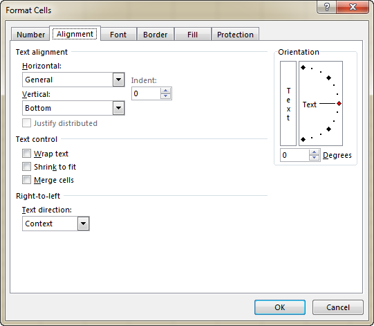
Another way to re-align cells in Excel is using the Alignment tab of the Format Cells dialog box. To get to this dialog, select the cells you want to align, and then either:
- Press Ctrl + 1 and switch to the Alignment tab, or
- Click the Dialog Box Launcher arrow at the bottom right corner of the Alignment

In addition to the most used alignment options available on the ribbon, the Format Cells dialog box provides a number of less used (but not less useful) features:

Now, let's take a closer look at the most important ones.
Text alignment options
Apart from aligning text horizontally and vertically in cells, these options allow you to justify and distribute the cell contents as well as fill an entire cell with the current data.

How to fill cell with the current contents
Use the Fill option to repeat the current cell content for the width of the cell. For example, you can quickly create a border element by typing a period in one cell, choosing Fill under Horizontal alignment, and then copying the cell across several adjacent columns:
![]()
How to justify text in Excel
To justify text horizontally, go to the Alignment tab of the Format Cells dialog box, and select the Justify option from the Horizontal drop-down list. This will wrap text and adjust spacing in each line (except for the last line) so that the first word aligns with the left edge and last word with the right edge of the cell:

The Justify option under Vertical alignment also wraps text, but adjusts spaces between lines so the text fills the entire row height:

How to distribute text in Excel
Like Justify, the Distributed option wraps text and "distributes" the cell contents evenly across the width or height of the cell, depending on whether you enabled Distributed horizontal or Distributed vertical alignment, respectively.
Unlike Justify, Distributed works for all lines, including the last line of the wrapped text. Even if a cell contains short text, it will be spaced-out to fit the column width (if distributed horizontally) or the row height (if distributed vertically). When a cell contains just one item (text or number without in-between spaces), it will be centered in the cell.
This is what the text in a distributed cell looks like:
Distributed horizontally |
Distributed vertically |
Distributed horizontally
|
 |
 |
 |
When changing the Horizontal alignment to Distributed, you can set the Indent value, telling Excel how many indent spaces you want to have after the left border and before the right border.
If you don't want any indent spaces, you can check the Justify Distributed box at the bottom of the Text alignment section, which ensures that there are no spaces between the text and cell borders (the same as keeping the Indent value to 0). If Indent is set to some value other than zero, the Justify Distributed option is disabled (grayed out).
The following screenshots demonstrate the difference between distributed and justified text in Excel:
Justified horizontally |
Distributed horizontally |
Justify distributed
|
 |
 |
 |
Tips and notes:
- Usually, justified and/or distributed text looks better in wider columns.
- Both Justify and Distributed alignments enable wrapping text In the Format Cells dialog, the Wrap text box will be left unchecked, but the Wrap Text button on the ribbon will be toggled on.
- As is the case with text wrapping, sometimes you may need to double click the boundary of the row heading to force the row to resize properly.
Center across selection
Exactly as its name suggests, this option centers the contents of the left-most cell across the selected cells. Visually, the result is indistinguishable from merging cells, except that the cells are not really merged. This may help you present the information in a better way and avoid undesirable side-effects of merged cells.

Text control options
These options control how your Excel data is presented in a cell.
Wrap text - if the text in a cell is larger than the column width, enable this feature to display the contents in several lines. For more information, please see How to wrap text in Excel.
Shrink to fit - reduces the font size so that the text fits into a cell without wrapping. The more text there is in a cell, the smaller it will appear.
Merge cells - combines selected cells into one cell. For more information, please see How to merge cells in Excel without losing data.
The following screenshots show all text control options in action.
Wrap text |
Shrink to fit |
Merge cells |
 |
 |
 |
Changing text orientation
The text orientation options available on the ribbon only allow to make text vertical, rotate text up and down to 90 degrees and turn text sideways to 45 degrees.
The Orientation option in the Format Cells dialog box enables you to rotate text at any angle, clockwise or counterclockwise. Simply type the desired number from 90 to -90 in the Degrees box or drag the orientation pointer.

Changing text direction
The bottom-most section of the Alignment tab, named Right-to-left, controls the text reading order. The default setting is Context, but you can change it to Right-to-Left or Left-to-Right. In this context, "right-to-left" refers to any language that is written from right to left, for example Arabic. If you don't have a right-to-left Office language version installed, then you will need to install an appropriate language pack.
How to change alignment in Excel with custom number format
For starters, it should be noted that the Excel number format is not explicitly designed for setting cell alignment. However, it allows "hardcoding" alignment for certain cells to ensure that your data looks exactly the way you want, regardless of the alignment options enabled on the ribbon. Please note, this method requires at least some basic knowledge of format codes, which are explained in detail in this tutorial: Custom Excel number format. Below I will demonstrate the general technique.
To set cell alignment with a custom number format, use the repeat characters syntax, which is nothing else but the asterisk (*) followed by the character you want to repeat, the space character in this case.
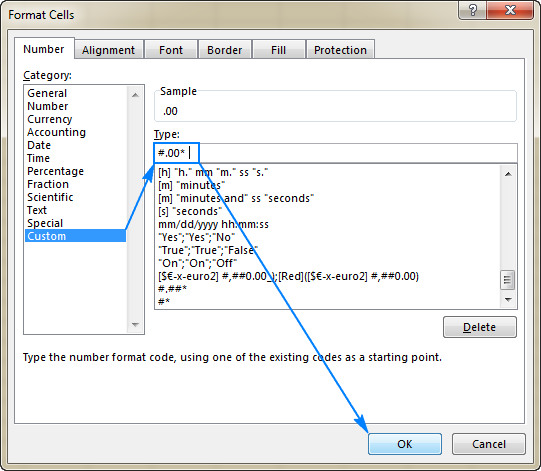
For example, to get numbers to align left in cells, take a regular format code that displays 2 decimal places #.00, and type an asterisk and a space at the end. As the result, you get this format: "#.00* " (double quotes are used only to show that an asterisk is followed by a space character, you don't want them in a real format code). If you want to display a thousand separator, use this custom format: "#,###* "
Taking a step further, you can force numbers to align left and text to align right by defining all 4 sections of the number format: positive numbers; negative numbers; zero; text. For instance: #,###* ; -#,###* ; 0* ;* @
With the format code established, perform the following steps to apply it:
- Select a cell(s) that you want to format.
- Press Ctrl + 1 to open the Format Cells
- Under Category, select Custom.
- Type your custom format code in the Type
- Click OK to save the newly created format.

Now, no matter what alignment options your users select on the ribbon, the data will be aligned according to the custom number format you've set:

Now that you know the essentials of Excel alignment, let me show you a couple of tips to enhance the visual presentation of your data.
How to align a column of numbers by decimal point in Excel
To align numbers in a column by decimal point, create a custom number format as explained in the above example. But this time, you will be using the "?" placeholder that leaves a space for insignificant zeros but does not display them.
For example, to align numbers in a column by decimal point and display up to 2 decimal places, you can use any of the following formats:
- #.?? - drops insignificant zeros to the left of the decimal point. For example, 0.5 will be displayed as .5
- 0.?? - shows one insignificant zero to the left of the decimal point.
- 0.0? - shows one insignificant zero on both sides of the decimal point. This format is best to be used if your column contains both integers and decimals (please see the screenshot below).
In the above format codes, the number of question marks to the right of the decimal point indicates how many decimal places you want to show. For instance, to display 3 decimal places, use #.??? or 0.??? or 0.0?? format.
If you want to align numbers to the left in cells and have the decimal points align, click the Align Left icon on the ribbon, and then apply a custom format similar to this: _-???0.0?;-???0.0?
Where:
- Semicolon (;) divides the format for positive numbers and zeros from the format for negative numbers.
- Underscore (_) inserts a whitespace equal to the width of a minus (-) character.
- The number of placeholders to the right of the decimal point determines the maximum number of decimal places to be displayed (2 in the above format).
- A question mark (?) to the left of the decimal point takes up a space equal to the width of one digit, if a digit is not present. So, the above format code will work for numbers that have up to 3 digits in the integer part. If you are dealing with bigger numbers, you will have to add more "?" placeholders.
The following screenshot shows the above custom number formats in action:

How to align numbers in a column by a specific character/symbol
In situations when the capabilities of Excel alignment may not be sufficient to replicate a certain data layout, Excel formulas may work a treat. To makes things easier to understand, let's consider the following example.
Goal: To have numbers centered in cells and aligned by the plus (+) symbol:

Solution: Create a helper column with the following formula, and then apply a monotype font like "Courier New" or "Lucida Sans Typewriter" to the helper column.
Where:
- cell - a cell containing the original string.
- char - a character you want to align by.
- n - the maximal number of characters before the aligning character, plus 1.
How this formula works: In essence, the formula adds leading spaces to the original string by repeating the space character, and then concatenates those spaces with the string. The number of spaces is calculated by subtracting the position of the aligning character from the maximum number of characters preceding it.
In this example, the formula takes the following shape:
=REPT(" ",12-FIND("+",A2))&A2
And works perfectly!

This is how you change cell alignment in Excel. I thank you for reading and hope to see you on our blog next week.
 by
by
15 comments
I have question.
How to allying cursor so I will start writing from the middle of the cell ?
Hello!
Select all target cells and choose Middle Align and/or Center on the Home tab, in the Alignment group.
I would like to change the default alignment once in option so I do not have to change it to my liking every time I create a new workbook.
Please guide me if that is posible.
Hello Johan!
Yes, you can set the default alignment in Excel so that it applies to all new workbooks you create. Here’s how you can do it:
Step 1: Open a new workbook in Excel. Format the alignment to your liking.
Step 2: Save the Workbook as a Template. Go to File > Save As. In the "Save as" type dropdown, select Excel Template (*.xltx).
Name your template (e.g., Book.xltx) and save it in the following folder: `C:\Users
\[Your Username]\AppData\Local\Microsoft\Excel\XLSTART`.
Step 3: Now, every time you open a new workbook, Excel will use this template and apply the default alignment settings you configured.
Read more: Excel templates: how to make and use.
Hey - Im trying to have a merged cell populate exactly as it is on another tab in my excel. I have the same amount of merged cells on both tabs, but I keep getting a "#spill" error when I put in "='Other Tab'!D8"
The text in the cell is left aligned and its much bigger than the cells that I need to be under it, so I need the cells either merged OR it would work if I could do something like "centre across selection" but still have it left justified.
Is there any way to either connect merged cells without getting a "spill" error OR wrap text at the end of a selection instead of only in one cell?
Hey, a reference to another cell cannot get that cell's formatting. I recommend reading this guide: #SPILL! error in Excel - what it means and how to fix.
1
3
0
7
HOW TO CHANGE TO 1307 IN CELL
Hi!
I recommend reading this guide: Merge and combine cells in Excel without losing data.
Or, if all of that text is in one cell (cell A1) you can use: =SUBSTITUTE(A1,CHAR(10),"")
Any Keyboard Shortcut to justify the Text in MS Excel 2010?
Hello!
The list of Keyboard shortcuts in Excel is available at this link
Is it possible to use autocorrect or conditional formatting to align text to centre in a cell? I cannot find a solution to this. For example, if a cell contains "n/a" I want the text to be centred in the cell.
Thanks a lot for the valuable information.
Shouldn't that be align ?
Definitely, it should. Don't know how these silly typos sneak in :) Thank you, Eric!