The tutorial explains the syntax and basic uses of the CHOOSE function and provides a few non-trivial examples showing how to use a CHOOSE formula in Excel.
CHOOSE is one of those Excel functions that may not look useful on their own, but combined with other functions give a number of awesome benefits. At the most basic level, you use the CHOOSE function to get a value from a list by specifying the position of that value. Further on in this tutorial, you will find several advanced uses that are certainly worth exploring.
Excel CHOOSE function - syntax and basic uses
The CHOOSE function in Excel is designed to return a value from the list based on a specified position.
The function is available in Excel 365, Excel 2019, Excel 2016, Excel 2013, Excel 2010, and Excel 2007.
The syntax of the CHOOSE function is as follows:
Where:
Index_num (required) - the position of the value to return. It can be any number between 1 and 254, a cell reference, or another formula.
Value1, value2, … - a list of up to 254 values from which to choose. Value1 is required, other values are optional. These can be numbers, text values, cell references, formulas, or defined names.
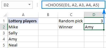
Here's an example of a CHOOSE formula in the simplest form:
=CHOOSE(3, "Mike", "Sally", "Amy", "Neal")
The formula returns "Amy" because index_num is 3 and "Amy" is the 3rd value in the list:
Excel CHOOSE function - 3 things to remember!
CHOOSE is a very plain function and you will hardly run into any difficulties implementing it in your worksheets. If the result returned by your CHOOSE formula is unexpected or not the result you were looking for, it may be because of the following reasons:
- The number of values to choose from is limited to 254.
- If index_num is less than 1 or greater than the number of values in the list, the #VALUE! error is returned.
- If the index_num argument is a fraction, it is truncated to the lowest integer.
How to use CHOOSE function in Excel - formula examples
The following examples show how CHOOSE can extend the capabilities of other Excel functions and provide alternative solutions to some common tasks, even to those that are considered unfeasible by many.
Excel CHOOSE instead of nested IFs
One of the most frequent tasks in Excel is to return different values based on a specified condition. In most cases, this can be done by using a classic nested IF statement. But the CHOOSE function can be a quick and easy-to-understand alternative.
Example 1. Return different values based on condition
Supposing you have a column of student scores and you want to label the scores based on the following conditions:
| Result | Score |
| Poor | 0 - 50 |
| Satisfactory | 51 - 100 |
| Good | 101 - 150 |
| Excellent | over 151 |
One way to do this is to nest a few IF formulas inside each other:
=IF(B2>=151, "Excellent", IF(B2>=101, "Good", IF(B2>=51, "Satisfactory", "Poor")))
Another way is to choose a label corresponding to the condition:
=CHOOSE((B2>=0) + (B2>=51) + (B2>=101) + (B2>=151), "Poor", "Satisfactory", "Good", "Excellent")

How this formula works:
In the index_num argument, you evaluate each condition and return TRUE if the condition is met, FALSE otherwise. For example, the value in cell B2 meets the first three conditions, so we get this intermediate result:
=CHOOSE(TRUE + TRUE + TRUE + FALSE, "Poor", "Satisfactory", "Good", "Excellent")
Given that in most Excel formulas TRUE equates to 1 and FALSE to 0, our formula undergoes this transformation:
=CHOOSE(1 + 1 + 1 + 0, "Poor", "Satisfactory", "Good", "Excellent")
After the addition operation is performed, we have:
=CHOOSE(3, "Poor", "Satisfactory", "Good", "Excellent")
As the result, the 3rd value in the list is returned, which is "Good".
Tips:
- To make the formula more flexible, you can use cell references instead of hardcoded labels, for example:
=CHOOSE((B2>=0) + (B2>=51) + (B2>=101) + (B2>=151), $E$1, $E$2, $E$3, $E$4) - If none of your conditions is TRUE, the index_num argument will be set to 0 forcing your formula to return the #VALUE! error. To avoid this, simply wrap CHOOSE in the IFERROR function like this:
=IFERROR(CHOOSE((B2>=0) + (B2>=51) + (B2>=101) + (B2>=151), "Poor", "Satisfactory", "Good", "Excellent"), "")
Example 2. Perform different calculations based on condition
In a similar fashion, you can use the Excel CHOOSE function to perform one calculation in a series of possible calculations/formulas without nesting multiple IF statements inside each other.
As an example, let's calculate the commission of each seller depending on their sales:
| Commission | Sales |
| 5% | $0 to $50 |
| 7% | $51 to $100 |
| 10% | over $101 |
With the sales amount in B2, the formula takes the following shape:
=CHOOSE((B2>=0) + (B2>=51) + (B2>=101), B2*5%, B2*7%, B2*10%)

Instead of hardcoding the percentages in the formula, you can refer to the corresponding cell in your reference table, if there is any. Just remember to fix the references using the $ sign.
=CHOOSE((B2>=0) + (B2>=51) + (B2>=101), B2*$E$2, B2*$E$3, B2*$E$4)
Excel CHOOSE formula to generate random data
As you probably know, Microsoft Excel has a special function to generate random integers between the bottom and top numbers that you specify - RANDBETWEEN function. Nest it in the index_num argument of CHOOSE, and your formula will generate almost any random data you want.
For example, this formula can produce a list of random exam results:
=CHOOSE(RANDBETWEEN(1,4), "Poor", "Satisfactory", "Good", "Excellent")
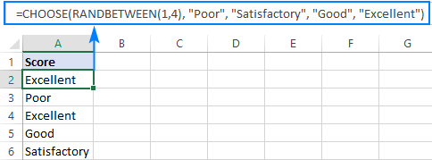
The formula's logic is obvious: RANDBETWEEN generates random numbers from 1 to 4 and CHOOSE returns a corresponding value from the predefined list of four values.
Note. RANDBETWEEN is a volatile function and it recalculates with every change you make to the worksheet. As the result, your list of random values will also change. To prevent this from happening, you can replace formulas with their values by using the Paste Special feature.
CHOOSE formula to do a left Vlookup
If you have ever performed a vertical lookup in Excel, you know that the VLOOKUP function can only search in the left-most column. In situations when you need to return a value to the left of the lookup column, you can either use the INDEX / MATCH combination or trick VLOOKUP by nesting the CHOOSE function into it. Here's how:
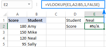
Supposing you have a list of scores in column A, student names in column B, and you want to retrieve a score of a particular student. Since the return column is to the left of the lookup column, a regular Vlookup formula returns the #N/A error:
To fix this, get the CHOOSE function to swap the positions of columns, telling Excel that column 1 is B and column 2 is A:
=CHOOSE({1,2}, B2:B5, A2:A5)
Because we supply an array of {1,2} in the index_num argument, the CHOOSE function accepts ranges in the value arguments (normally, it doesn't).
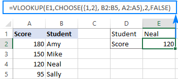
Now, embed the above formula into the table_array argument of VLOOKUP:
=VLOOKUP(E1,CHOOSE({1,2}, B2:B5, A2:A5),2,FALSE)
And voilà - a lookup to the left is performed without a hitch!
CHOOSE formula to return next working day
If you are not sure whether you should go to work tomorrow or can stay at home and enjoy your well-deserved weekend, the Excel CHOOSE function can find out when the next work day is.
Assuming your working days are Monday to Friday, the formula goes as follows:
=TODAY()+CHOOSE(WEEKDAY(TODAY()),1,1,1,1,1,3,2)

Tricky at first sight, upon a closer look the formula's logic is easy to follow:
WEEKDAY(TODAY()) returns a serial number corresponding to today's date, ranging from 1 (Sunday) to 7 (Saturday). This number goes to the index_num argument of our CHOOSE formula.
Value1 - value7 (1,1,1,1,1,3,2) determine how many days to add to the current date. If today is Sunday - Thursday (index_num 1 - 5), you add 1 to return the next day. If today is Friday (index_num 6), you add 3 to return next Monday. If today is Saturday (index_num 7), you add 2 to return next Monday again. Yep, it's that simple :)
CHOOSE formula to return a custom day/month name from date
In situations when you want to get a day name in the standard format such as full name (Monday, Tuesday, etc.) or short name (Mon, Tue, etc.), you can use the TEXT function as explained in this example: Get day of week from date in Excel.
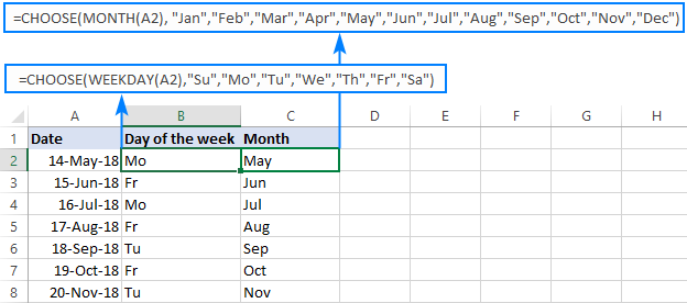
If you wish to return a day of the week or a month name in a custom format, use the CHOOSE function in the following way.
To get a day of the week:
=CHOOSE(WEEKDAY(A2),"Su","Mo","Tu","We","Th","Fr","Sa")
To get a month:
=CHOOSE(MONTH(A2), "Jan","Feb","Mar","Apr","May","Jun","Jul","Aug","Sep","Oct","Nov","Dec")
Where A2 is the cell containing the original date.
I hope this tutorial has given you some ideas of how you can use the CHOOSE function in Excel to enhance your data models. I thank you for reading and hope to see you on our blog next week!
 by
by
17 comments
When look at the post, the Array is distorted from the spacing I used in the comment box. Hopefully you can still understand it. A,B,C,D are the columns and 1,2,3,4 are the row numbers. The numbers 50,60,70 and 80 should be under A,B,C,D respectively and then the numbers 1 to 16 below that. The numbers 10,20,30 and 40 should be to the right of the row numbers 1,2,3,4. So the number 7 that I am trying to put into Cell3 would be from row 2 (variable1= 20) and column C (variable2 = 70) Hope this helps...
I have Variable1 in Cell1 and Variable2 in Cell2. Variable1 can be 10,20,30 or 40. Variable2 can be 50,60,70 or 80.
If Variable1 = 20 and Variable2 =70, how do I return the value 7 into a Cell3 from the array shown here (A,B,C,D are columns and 1,2,3,4 are rows)
A B C D
50 60 70 80
1 10 1 2 3 4
2 20 5 6 7 8
3 30 9 10 11 12
4 40 13 14 15 16
thank you for your help with this....
Hello Baden!
The answer to your question can be found in this article: Excel INDEX MATCH MATCH and other formulas for two-way lookup.
"Left lookup" tab in "practice workbook" availabe for download there is formula:
=VLOOKUP(E1;CHOOSE({1\2}; B2:B5; A2:A5);2;FALSE)
The text above (section "CHOOSE formula to do a left Vlookup") is showing formula, which is not working in my Excel 2021:
=VLOOKUP(E1,CHOOSE({1,2}, B2:B5, A2:A5),2,FALSE)
So there is obviously significant difference between "\" and ",". And yes, I am using ";" as delimiter.
Anyhow, thank you very much for this article.
Hi! It depends on your computer's regional settings.
hi friends
i need help!
i have 27 people that need to be assigned to their 1, 2, 3, 4th choices for a critique session. They are already ordered by timestamp. The trick is that there are 8 choices, in total. Help???
Hi! Unfortunately, this information is not enough to recommend a formula to you. I'd recommend you to take a look at our Random Generator tool. It is available as a part of our Ultimate Suite for Excel that you can install in a trial mode and check how it works for free.
How can I use vlookup with choose between 2 worksheets .?
Hi! If I understand the question correctly, the formula might look something like this:
CHOOSE(D1,VLOOKUP(lookup_value, Sheet_1!range, col_index_num, [range_lookup]), VLOOKUP(lookup_value, Sheet_2!range, col_index_num, [range_lookup]))
For more information, please visit: How to VLOOKUP across multiple sheets in Excel.
Create an efficient formula in range G2:G21 that gives a decision for each customer with either the text “Extend Credit” or “No Credit.” Copy this formula down for each customer.
What formula would I use? How to enter in cell "Extend Credit" or "No credit"?
Why it always says ''error'' when i put 5 choices?
I also get an error but I'm using 4 choices.
Hi,
I need help to all of you
actually i am creating a incentive calculator for my Sales team
according to our incentive policy
if a sales person achive his monthly target then the total unit multiply with the rate,
here is 2 different situation apply
1st situation
if a person achive his monthly target >100%
for example
a person sale a product 110unit
100 unit is a monthly target
the 100 unit multiply with 100% slab and rest of the 10 unit multiply with >100% or 110% slab.
the slab are also mention here
<80% <89% <99% 100% 110%
56 62.3 69.3 70 87.5 105
kindly suggest me some better option for the calculating of these incentive
Faisal:
If I understand your question here's the formula for the calculation:
=IF(M32<=80,(M32*56),IF(M32<=89,(M32*62.3),IF(M32<=99,(M32*69.3),IF(M32100,(M32*87.5))))))
Enter this into an empty cell and enter the achieved amount in M32. If you want to enter the achieved amount in another cell, change the "M32" addresses in the formula to that cell's address.
You can both simplify the formula and "improve" it by "dynamic coding".
The following formula:
=CHOOSE((B2>0)+(B2>=51)+(B2>=101)+(B2>=151),$E$1,$E$2,$E$3,$E$4)
is better than:
=CHOOSE((B2>0)+(B2>=51)+(B2>=101)+(B2>=151),"Poor", "Satisfactory", "Good", "Excellent")
A reference to a cell is always better than "hard coding".
The same principle applies to the commission example, too.
Best Regards,
Meni Porat
you are right, but it is often said that for high volumes of data it is better to use constants in formulas than references