How to convert column number to letter in Excel

How to convert column number into alphabet (single-letter columns)

In case the column name consists of a single letter, from A to Z, you can get it by using this simple formula:

For example, to convert number 10 to a column letter, the formula is:

=CHAR(64 + 10)

It's also possible to input a number in some cell and refer to that cell in your formula:

=CHAR(64 + A2)

How this formula works:

The CHAR function returns a character based on the character code in the ASCII set. The ASCII values of the uppercase letters of the English alphabet are 65 (A) to 90 (Z). So, to get the character code of uppercase A, you add 1 to 64; to get the character code of uppercase B, you add 2 to 64, and so on.

How to convert Excel column number to letter (any column)

If you are looking for a versatile formula that works for any column in Excel (1 letter, 2 letter and 3 letter), then you'll need to use a bit more complex syntax:

With the column letter in A2, the formula takes this form:

=SUBSTITUTE(ADDRESS(1, A2, 4), "1", "")

How this formula works:

First, you construct a cell address with the column number of interest. For this, supply the following arguments to the ADDRESS function:

• 1 for row_num (the row number does not really matter, so you can use any).
• A2 (the cell containing the column number) for column_num.
• 4 for abs_num argument to return a relative reference.

With the above parameters, the ADDRESS function returns the text string "A1" as the result.

As we only need a column letter, we strip the row number with the help of the SUBSTITUTE function, which searches for "1" (or whatever row number you hardcoded inside the ADDRESS function) in the text "A1" and replaces it with an empty string ("").

Get column letter from column number using custom function Custom function

If you need to convert column numbers into alphabetical characters on a regular basis, then a custom user-defined function (UDF) can save your time immensely.

The code of the function is pretty plain and straightforward:

Here, we use the Cells property to refer to a cell in row 1 and the specified column number and the Address property to return a string containing an absolute reference to that cell (such as $A$1). Then, the Split function breaks the returned string into individual elements using the $ sign as the separator, and we return element (1), which is the column letter.

Paste the code in the VBA editor, and your new ColumnLetter function is ready for use. For the detailed guidance, please see: How to insert VBA code in Excel.

From the end-user viewpoint, the function's syntax is as simple as this:

Where col_num is the column number that you want to convert into a letter.

Your real formula can look as follows:

=ColumnLetter(A2)

And it will return exactly the same results as native Excel functions discussed in the previous example:

How to get column letter of certain cell

To identify a column letter of a specific cell, use the COLUMN function to retrieve the column number, and serve that number to the ADDRESS function. The complete formula will take this shape:

As an example, let's find a column letter of cell C5:

=SUBSTITUTE(ADDRESS(1, COLUMN(C5), 4), "1", "")

Obviously, the result is "C" :)

How to get column letter of the current cell

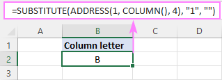
To work out the letter of the current cell, the formula is almost the same as in the above example. The only difference is that the COLUMN() function is used with an empty argument to refer to the cell where the formula is:

=SUBSTITUTE(ADDRESS(1, COLUMN(), 4), "1", "")

How to create dynamic range reference from column number

Hopefully, the previous examples have given you some new subjects for thought, but you may be wondering about the practical applications.

In this example, we'll show you how to use the "column number to letter" formula for solving real-life tasks. In particular, we'll create a dynamic XLOOKUP formula that will pull values from a specific column based on its number.

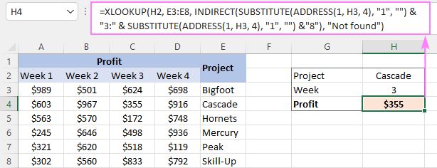
From the sample table below, suppose you wish to get a profit figure for a given project (H2) and week (H3).

To accomplish the task, you need to provide XLOOKUP with the range from which to return values. As we only have the week number, which corresponds to the column number, we are going to convert that number to a column letter first, and then construct the range reference.

For convenience, let's break down the whole process into 3 easy to follow steps.

1. Convert a column number to a letter

   With the column number in H3, use the already familiar formula to change it to an alphabetical character:

   =SUBSTITUTE(ADDRESS(1, H3, 4), "1", "")
   

   Tip. If the number in your dataset does not match the column number, be sure to make the required correction. For example, if we had the week 1 data in column B, the week 2 data in column C, and so on, then we'd use H3+1 to get the correct column number.

2. Construct a string representing a range reference

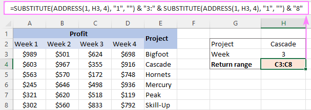
   To build a range reference in the form of a string, you concatenate the column letter returned by the above formula with the first and last row numbers. In our case, the data cells are in rows 3 through 8, so we are using this formula:

   =SUBSTITUTE(ADDRESS(1, H3, 4), "1", "") & "3:" & SUBSTITUTE(ADDRESS(1, H3, 4), "1", "") & "8"

   Given that H3 contains "3", which is converted to "C", our formula undergoes the following transformation:

   ="C"&"3:"&"C"&"8"

   And produces the string C3:C8.
   

3. Make a dynamic range reference

   To transform a text string into a valid reference that Excel can understand, nest the above formula in the INDIRECT function, and then pass it to the 3^rd argument of XLOOKUP:

   =XLOOKUP(H2, E3:E8, INDIRECT(H4), "Not found")
   

   To get rid of an extra cell containing the return range string, you can place the SUBSTITUTE ADDRESS formula within the INDIRECT function itself:

   =XLOOKUP(H2, E3:E8, INDIRECT(SUBSTITUTE(ADDRESS(1, H3, 4), "1", "") & "3:" & SUBSTITUTE(ADDRESS(1, H3, 4), "1", "") & "8"), "Not found")
   

With our custom ColumnLetter function, you can get a more compact and elegant solution:

=XLOOKUP(H2, E3:E8, INDIRECT(ColumnLetter(H3) & "3:" & ColumnLetter(H3) & "8"), "Not found")

Practice workbook for download

Excel column number to letter - examples (.xlsm file)