The article looks at how to quickly turn a cell range into a table using the default or selected table style and how to undo a table so it changes back to a normal range.
Table is one of the most useful things in Excel that makes managing, calculating and updating data a lot easier. Under certain circumstances, however, a table format may not suit your needs. Luckily, there is a quick way to turn a table into a normal range without losing your data. And the other way round, you can easily transform a cell range to a fully-functional table whenever you need it.
Excel table vs. range: what's the difference?
Among Excel users, especially beginners, there's a lot of confusion and uncertainty about the terms range and table. When you input some data in a worksheet, can you already call your dataset a table? Many people do so. From Excel's viewpoint, however, it's a range, not a table. So, what's the difference?
Range in Excel means any group of selected cells. It is defined by the reference of the top-left cell and the bottom-right cell. For example, in the left-hand part of the image below, the data is in the range A1:C6.
Excel table is a structured and pre-formatted dynamic range of cells that has its own name. You can think of a table as an advanced version of range with inbuilt functionality such as calculated columns, banded rows, sorting and filtering, etc. We say that a table is dynamic because it expands automatically as you add new data to it.
You can easily identify a table in an Excel worksheet due to these noticeable features: table data is always surrounded by a thin border like shown in the right-hand part of the image below. Auto-filter arrows appear next to the column headers, and the headings remain frozen at the top when you scroll through the data.

For more information, please see Excel table: comprehensive tutorial with examples.
Why would you want to convert a range into an Excel table?
Turning a range of cells into a fully functional Excel table extends its functionality with many advanced features that can take your spreadsheets to a new level:
What does it mean to convert an Excel table to a range?
Microsoft Excel allows quickly transforming a table back to a normal range. This will remove all of the table features but keep table style formatting. Below, you'll find detailed guidance on how to do that.
How to convert a table to a range in Excel
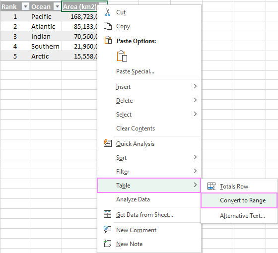
The fastest way to transform the table into a normal range is this: right-click any cell in your table, and then click Table > Convert to Range.

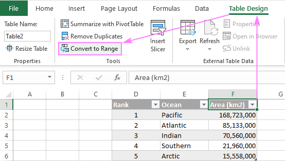
You can also undo a table in Excel using the ribbon menu:
- Select any cell in the table to activate the Table Design tab.
- On the Table Design tab, in the Tools group, click Convert to Range.

Either way, Excel will display a prompt asking you to confirm your intention:

Once you click Yes, the table is immediately changed backed to a normal range of cells:

Note. This method changes a table to a usual range and removes all features of an Excel table such as automatic expansion, structured references, filter buttons, etc. However, it does keep the table style formatting such as fill and font colors, borders, and the like. If you don't want it, remove table formatting before converting the table to a range.
How to convert data range to a table
If you'd like to leverage many wonderful features included with the Excel table format, you can turn your current data into a fully-fledged table by using one of the following approaches.
Convert range to table in Excel
The quickest way to convert a data range to a table is this:
- Select any cell in your dataset and press the Ctrl + T keys together.
- The Create Table dialog box will pop-up. Here, you just verify if Excel has picked your data range correctly, make sure the My table has headers box is selected (if your dataset does not have headers, then of course unselect it), and click OK.

That's it! The selected range is converted to a table right away:

Tip. This method creates a table with the default style. You can change it at any moment by picking another style from the Table Styles gallery. For more information, please see How to change table style in Excel.
Another way to turn a range into a table
As is often the case in Excel, a command performed with a keyboard shortcut is also accessible from the ribbon. So, here's one more way to create a table in Excel:
- Select your dataset or any single cell within it.
- Head over to the Insert tab > Tables group and click Table.

- In the Create Table dialog box that pops up, verify the selected range, check or uncheck the My table has headers box, and click OK.
Tip. Like the previous method, this one also creates a table using the default style. To control which style is applied to your table, use the bellow approach.
Convert the cell range to a table using table style
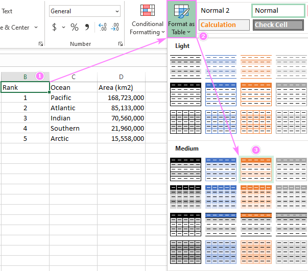
To change a range to a table using the style you like best, these are the steps to perform:
- Select any cell in your data set.
- On the Home tab, in the Styles group, click Format as Table.
- Pick the desired table style in the gallery.
- In the Create Table dialog box, make sure the selected range if correct and the My table has headers box is checked, and then click OK.

As the result, the selected range gets converted to a table with the style of your choosing:

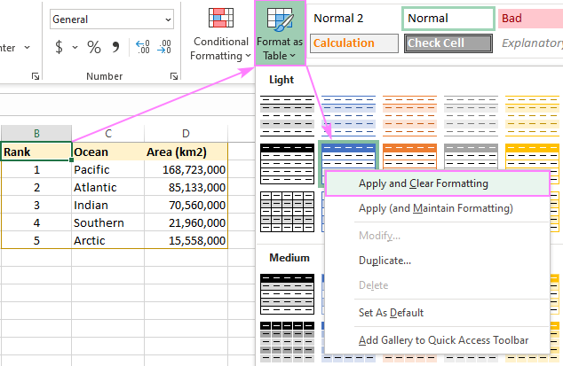
If your dataset already has some cell formatting and you do not want it to get messed up with the inbuilt table style, then right-click the style in the gallery and choose Apply and Clear Formatting. This will remove all existing formatting from the range, and then apply the selected table style.

Tip. To swiftly transform a selected range into a table, you can also use the Quick Analysis Tables feature.
That's how to convert a range to a table in Excel and change it back to a normal cell range. I thank you for reading and look forward to seeing you on our blog next week!
 by
by
One comment
It is helpfull