In this tutorial, you will learn a few different ways of copying formulas in Excel - how to copy formula down a column, to all of the selected cells, copy a formula exactly without changing cell references or formatting, and more.
Copying formulas in Excel is one of the easiest tasks that is usually done in a mouse click. I say "usually" because there can be very specific cases that require special tricks, like copying a range of formulas without changing cell references or entering the same formula in multiple non-adjacent cells.
Luckily, Microsoft Excel offers many ways to do the same task, and it is true for copying formulas. In this tutorial, we are going to discuss different ways to copy formulas in Excel so that you could choose the one best suited for your task.
How to copy formula down a column
Microsoft Excel provide a really quick way to copy a formula down a column. You just do the following:
- Enter a formula in the top cell.
- Select the cell with the formula, and hover the mouse cursor over a small square at the lower right-hand corner of the cell, which is called the Fill handle. As you do this, the cursor will change to a thick black cross.
- Hold and drag the fill handle down the column over the cells where you want to copy the formula.
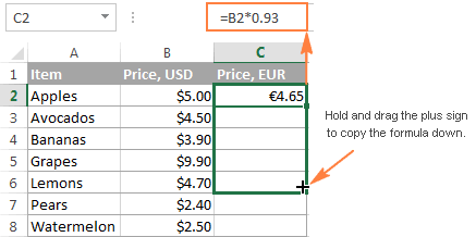
In a similar manner, you can drag formula into adjacent cells to the right, to the left or upwards.
If the formula includes relative cell references (without the $ sign), they will automatically change based on a relative position of rows and columns. So, after copying the formula, verify that the cell references have got adjusted properly and produce the result that you want. If necessary, switch between absolute, relative and mixed references by using the F4 key.
In the above example, to make sure the formula was copied correctly, let's select some cell in column C, say C4, and view the cell reference in the formula bar. As you can see in the screenshot below, the formula is all right - relative to row 4, exactly as it should be:

How to copy a formula down without copying formatting
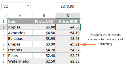
Copying a formula down by dragging the fill handle not only copies the formula, but also the source cell formatting such as font or background color, currency symbols, the number of displayed decimal places, etc. In most cases, this works just fine, but sometimes it can mess up the existing formats in cells where the formula is being copied to. A common example is overwriting alternate row shading like in the following screenshot.
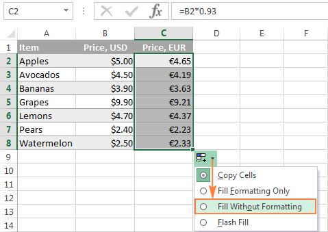
For prevent overwriting the existing cell formatting, drag the fill handle as demonstrated above, release it, click the Auto Fill Options drop-down menu, and select Fill Without Formatting.
Copy formula to the entire column
As you've just seen, the fill handle makes copying formulas in Excel really easy. But what if you need to copy a formula down a ten-hundred-line sheet? Dragging the formula over hundreds of rows does not look like a good idea. Luckily, Microsoft Excel provides a couple of quick solutions for this case as well.
Double-click the plus sign to fill the whole column
To apply the formula to the entire column, double-click the plus sign instead of dragging it. For those who have skipped the first section of this tutorial, the detailed steps follow below.
To copy an Excel formula to the whole column, do the following:
- Input your formula in the top cell.
- Position the cursor to the lower right corner of the cell with the formula, wait until it turns into the plus sign, and then double-click the plus.

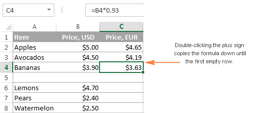
Note. Double-clicking the plus sign copies the formula down as far as there is some data in the adjacent column(s). As soon as an empty row occurs, the auto fill stops. So, if your worksheet contains any gaps, you will have to repeat the above process to copy the formula below an empty row or drag the fill handle as explained in the previous examples:
Create an Excel table to copy a formula to all cells in a column automatically
Among other great features of Excel tables such as predefined styles, sorting, filtering and banded rows, automatically calculated columns is what makes an Excel table a truly wonderful tool for analyzing groups of related data.
By entering a formula into one cell in a table column (just any cell, not necessarily the top one), you create a calculated column and have your formula instantly copied to all other cells in that column. Unlike the fill handle, Excel tables have no problem with copying the formula across the entire column even if the table has one or more empty rows:
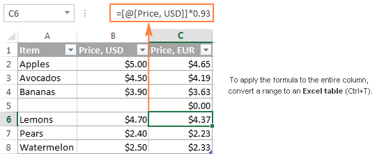
To convert a range of cells to an Excel table, simply select all the cells and press Ctrl + T. If you prefer a visual way, select the range, go to the Insert tab > Tables group on the Excel ribbon, and click the Table button.
Tip. If you don't really want an Excel table in your worksheet, to can create it temporary, to make the work with formulas easier, and then you can convert the table back to a usual range in a second. Just right-click the table and choose Table > Convert to Range in the context menu.
Copy a formula to non-adjacent cells / ranges
It goes without saying that the fill handle is the fastest way to copy formula in Excel. But what if you want to copy your Excel formula in non-contiguous cells or beyond the end of the source data? Just use the old good copy & paste way:
- Click the cell with the formula to select it.
- Press Ctrl + C to copy the formula.
- Select a cell or a range of cells where you want to paste the formula (to select non-adjacent ranges, press and hold the Ctrl key).
- Press Ctrl + V to paste the formula.
- Press Enter to complete the pasted formulas.

Note. The copy/paste shortcuts copy the formula and formatting. To copy the formula without formatting, choose an appropriate Paste option on the ribbon or in the right-click menu, as demonstrated in Copying an Excel formula without formatting.
Enter a formula into multiple cells with a single key stroke (Ctrl + Enter)
In situations when you need to input the same formula in more than one cell on a worksheet, adjacent or non-adjacent ones, this method can be a time-saver.
- Select all the cells where you want to enter the formula. To select non-contiguous cells, press and hold the Ctrl key.
- Press F2 to enter the edit mode.
- Input your formula in one cell, and press Ctrl + Enter instead of Enter. That's it! The formula will get copied to all of the selected cells, and Excel will adjust relative cell references accordingly.
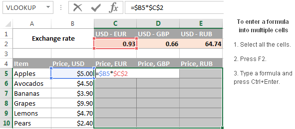
Tip. You can use this method to enter any data, not just formulas, in multiple cells at a time. A few other techniques are described in the following tutorial: How to enter the same data into all selected cells at a time.
How to copy an Excel formula but not formatting
As you already know, when copying a formula down a column in Excel, you can use the Fill Without Formatting option that lets you copy the formula but keep the existing formatting of the destination cells. Excel's Copy & Paste feature offers even more flexibility with regard to paste options.
- Select the sell containing the formula.
- Copy that cell by pressing Ctrl + C. Alternatively, right click the cell and select Copy from the context menu, or click the Copy button on the Home tab > Clipboard.
- Select all the cells to which you want to copy the formula.
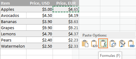
- Right-click the selected cells and choose Formulas under Paste Options:
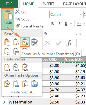
For more paste options, click the arrow below the Paste button on the ribbon. For example, you can select Formulas & Number Formatting to paste only the formula and the number formatting such as percent format, currency format, and the like:
Tip. If you are not sure which paste option works best for you, hover the mouse over different icons to see a preview of this or that paste option.
Copy formula in Excel without changing references
Excel formulas rarely occur in a spreadsheet in solitude. In most cases, you enter a formula in one cell, and then copy it to other cells in the same column or row, to perform the same calculation on a group of data. And if your formula contains relative cell references (without $), Excel automatically adjusts them so that each formula operates on data on its own row or column. Most of the time, this is exactly what you want. For example, if you have the formula =A1*2 in cell B1, and you copy this formula to cell B3, the formula will change to =A3*2.
But what if you want Excel to copy the formula exactly, without changing the cell references along the way? Depending on your particular task, choose one of the following solutions.
Copy or move a single formula without changing cell references
If you need to copy or move just one formula, making an exact copy is easy.
- Select the cell with the formula you want to copy.
- Select the formula in the formula bar using the mouse, and press Ctrl + C to copy it. If you want to move the formula, press Ctrl + X to cut it.
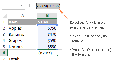
- Press the Esc key to exit the formula bar.
- Select the destination cell and press Ctl + V to paste the formula there.
Alternatively, you can enter the editing mode and copy the formula in the cell as text:
- Select a cell with the formula.
- Press F2 (or double-click the cell) to enter the editing mode.
- Select the formula in the cell using the mouse, and press Ctrl + C to copy it.
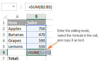
- Select the destination cell, and press Ctl+V. This will paste the formula exactly, without changing the cell references, because the formula was copied as text.
Tip. To quickly copy a formula from the above cell with no reference changed, select the cell where you want to paste the formula and press Ctrl + '.
Copy a range of formulas without changing cell references
To move or copy a range of Excel formulas so that no cell references are changed, use one of the following methods.
Method 1. Use absolute or mixed cell references
If you need to make an exact copy of formulas with relative cell references (like A1), the best way would be changing them to absolute references ($A$1) to fix the reference to a given cell, so that it remains static no matter where the formula moves. In other cases, you may need to use mixed cell references ($A1 or A$1) to lock either a column or row. Doesn't make much sense so far? Okay, let's consider the following example.
Supposing, you have a table that calculates the fruit prices in EUR based on the USD price in column B and the exchange rate in cell C2:

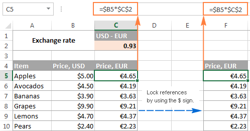
As you can see in the screenshot above, the formula includes an absolute cell reference ($C$2) to fix the exchange rate to cell C2, and a relative cell reference to cell B5 because you want this reference to adjust for each row. And this approach works well as long as the formulas remain in column C.
But let's see what happens if you need, say, to move the EUR prices from column C to column F. If you copy the formulas in a usual way by copying/pasting the cells, the formula from cell C5 (=B5*$C$2) will change to =D5*$C$2 when pasted in cell F5, making your calculations all wrong!
To fix this, just change a relative reference (B5) to a mixed reference $B5 (absolute column and relative row). By putting the dollar sign ($) in front of the column letter you anchor the reference to column B, no matter where the formula moves.
And now, if you copy or move the formulas from column D to column F, or any other column, the column reference won't change because you locked it by the dollar sign ($B5).
The concept of Excel cell references may be difficult to grasp from the outset, but trust me it's worth your time and effort because it will save you much more time in the long run. For example, see how you can calculate the entire table with a single formula by using mixed cell references.
However, if you already have a ton of formulas with relative cell references in your Excel sheet, and you need to quickly make an exact copy of those formulas but you don't feel like you can get the references right, one of the following methods could be a solution.
Method 2. Copy Excel formulas without changing references via Notepad
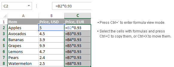
- Enter the formula view mode by pressing the Ctrl + ` shortcut, or by using any other method described in How to show formulas in Excel.
- Select all the cells with the formulas you want to copy or move.
- Press Ctrl + C to copy the formulas, or Ctrl + X to cut them. Use the latter shortcut if you want to move formulas to a new location.
- Open Notepad or any other text editor and press Ctrl + V to paste the formulas there. Then press Ctrl + A to select all the formulas, and Ctrl + C to copy them as text.
- In your Excel worksheet, select the upper-left cell where you want to paste the formulas, and press Ctrl + V.
Notes:
- You can paste the formulas only in the same worksheet where your original formulas are located, unless the references include the sheet name, otherwise the formulas will be broken.
- The worksheet should be in formula view mode. To verify this, go to the Formulas tab > Formula Auditing group, and check if the Show Formulas button is toggled on.
- After pasting the formulas, press Ctrl + ` to toggle off the formula view mode.
Method 3. Copy formulas exactly by using Excel's Find and Replace
To copy a range of Excel formulas without changing their cell references, you can use the Excel Find and Replace feature in the following way.
- Select the cells with the formulas that you want to copy.
- On the Home tab, go to the Editing group, and click Find & Select > Replace… Or, simply press Ctrl + H, which is the shortcut for launching the Find & Replace dialog in Excel.
- In the Find & Replace dialog window, type the equal sign (=) in the Find what box. In the Replace with box, input some symbol or a string of characters that is not used in any of your formulas, like ', # or \.
 The purpose of this step is to turn formulas into text strings, which will prevent Excel from changing the cell references during the copy process.
Note. Do not use an asterisk (*) or question mark (?) for replacement, since these are wildcard characters in Excel and using them would make later steps more difficult.
- Click the Replace All button and close the Find and Replace dialog. All the formulas in the selected range will turn into text strings:

- Now, you can select any cells, press Ctrl + C to copy them, select the top cell in the current worksheet where you want to paste the formulas, and press Ctrl + V. Since Excel does not interpret the formulas without the equal sign as formulas, they will be copied exactly, without changing references.
- Use Find & Replace again to reverse the change. Select both regions, with the original formulas and copied ones (to select non-adjacent regions, press and hold Ctrl). Press Ctrl + H to open the Find & Replace dialog. This time, enter the back slash (\) (or any other character you used for the first replacement) in the Find what box, and = in the Replace with box, and click the Replace All button. Done!
Shortcuts to copy Excel formula to other cells
1. Copy a formula down
Ctrl + D - Copy a formula from the cell above and adjusts the cell references.
For example, if you have a formula in cell A1 and you want to copy it to cell A2, select A2 and press Ctrl + D.

2. Copy a formula to the right
Ctrl + R - Copy a formula from the cell to the left and adjusts the cell references.
For example, if you have a formula in cell A2 and you want to copy it to cell B2, select B2 and press Ctrl + R.

Tip. Both of the above shortcuts can be used to copy formulas to multiple cells too. The trick is to select both the source cell and target cells before pressing the shortcut. For example, if you want to copy the formula from A1 to the next 9 rows, select cells A1:A10 and press Ctrl + D.
3. Copy a formula down exactly
Ctrl + ' - Copies a formula from the cell above to the currently selected cell exactly and leaves the cell in edit mode.
This is a quick way to make an exact copy of a formula without changing cell references. For example, to copy a formula from cell A1 to A2 so that no references are changed, select A2 and press Ctrl + '.
Note. Don't confuse the shortcut Ctrl + ' (Ctrl + single quote) that exactly copies a formula from the cell above with Ctrl + ` (Ctrl + grave accent key) that activates show formulas mode in Excel.

Well, this is all I have to say about copying formulas in Excel. If you know some other methods to quickly move or copy formula in Excel sheets, please do share. I thank you for reading and hope to see you on our blog next week!
 by
by
205 comments
You can copy formulas without changin references using the clipboard )instead of notepad)
1. Enter the formula view mode by pressing the Ctrl + ` shortcut, or by using any other method described in How to show formulas in Excel.
2. Select all the cells with the formulas you want to copy or move.
3. Press Ctrl + C to copy the formulas
4. Select the upper left corner of the destination
5. Open the clipboard (by clicking on the arrow in the clipboard group)
6. Select paste of the appropriate element of the clipboard. The exact formulas (no reference updates) are pasted on the dstination.
7. Exit the formula view mode by pressing the Ctrl + ` shortcut, or by using any other method described in How to show formulas in Excel.
Hello.
I am trying to copy a formula from d33. It is =D28*$G$12. Now I want to copy that formula to E34. It should be taking E28*$G$12 but it is taking D29 instead. Can you help with this?
Hi! Your question contains incorrect information. If you copy this formula from D33 to E34, you will get the formula =E29*$G$12.
Study carefully the recommendations in the article above as well as these instructions: Why use $ in Excel formula: relative & absolute cell reference.
Maybe this formula suits you:
=D$28*$G$12
I am trying to make a formula that I can autofill down (ex C2-C15) but I want the formula to only change by column (ex c2-c15 references B10-23).
How do I make excel do that? It’s also a complicated sum with some ranges and some individual cells.
I need to do this 24x 7 times on 7 different sheets, so I expect I’ll have to set up the first on each worksheet but I’d like to be able to just double click the + so it autofills the formula down.
Thank you.
Hi! If I understand your task correctly, the following tutorial should help: Relative and absolute cell reference: why use $ in Excel formula.
Is there a way to copy a subtotal formula when the number of rows that are being totaled are different?
Hello Jennifer!
When you copy a SUBTOTAL formula that references a cell range, the size of the cell range will not be changed. The same is true of any other Excel formula.
I need to add cells from one sheet into another and I would like to copy the formula. However, when I copy it instead of going from A1+A2 to A3+A4 it goes A1+A2 to A2+A3
Hi! Pay attention to the following paragraph of the article above: Copy a range of formulas without changing cell references.
It covers your case completely.
I am facing another problem. I am trying to use conditional formatting based on the multiplication of two cells being greater than the value in another cell. Apologies to post another question here but I have tried searching this and using various approaches but I can't seem to find anything that works.
Example:
If the sum of C4*D4 = greater than value in F1, then C4 and D4 highlight red. If no entry has been made or total is lower than that in F1 then cells are not highlighted.
Here is where I am at with the formula. I'm not receiving any error to fix but it is highlighting red when the total is lower than F1.
=IF(C4,",",SUM(C4*D4))>$F$1
Please can you advise me on where I'm going wrong or confirm if this is not possible to achieve.
Thank you.
Hi! You must create conditional formatting rule with formula: =$C1*$D1>$F$1
Read more: Excel conditional formatting formulas based on another cell and Relative and absolute cell references in Excel conditional formatting.
Brilliant! That works perfectly!
Thank you so much. I spent so long trying all kinds of different formulas and google searches!
Sorry, I have one more question I am hoping someone can help me with please.
I am trying to highlight a cell when the number has seen two consecutive reductions in the previous columns and I then need to apply this to the entire sheet (e.g. range D3:BS1) updating the references
e.g. D3=20, E3=19 and F3=18 then I would need F3 to highlight red.
if D3=20, E3=21, F3=19, G3=18 then no highlight would be necessary unless H3= <18.
Hope this makes sense!
Any help is appreciated.
Thank you.
Hi! You can create conditional formatting for the range F3:BS1 using this formula:
=AND(F1-OFFSET(F1,0,-1)=-1, OFFSET(F1,0,-1)-OFFSET(F1,0,-2)=-1)
The OFFSET function extracts values from the two cells to the left of F1 and compares them. You can find the examples and detailed instructions here: Excel OFFSET function - formula examples and uses.
Thanks so much, Alexander!
I have been playing around with this and looking at the detailed instructions you included, but I can only get the formula to highlight if the value has decreased each time by 1 and not by e.g. 2 or 3. Is there a simple adjustment to the formula that can highlight when the number has seen two consecutive reductions of >= 0.5 so for example, D3=20, E3=19.5, F3=16.2 then F3 is highlighted.
I appreciate the help!
Thank you.
Hi! Replace in the formula =-1 to >= 0.5
Thank you, Alexander.
I have tried this but can't seem to get it to work. Please can you advise on where I'm going wrong, or if you need more information.
Formula I am using: =AND(F36-OFFSET(F36,0,-1)>=0.5, OFFSET(F36,0,-1)-OFFSET(F36,0,-2)>=0.5)
In this case, the cell value of D36=20, E36=19.4, F36= 18.1 so the aim is for F36 to highlight but this is not happening.
Thanks for your help!
Hello, I am trying to copy a formula across multiple columns where I need the cell reference (captured from the measurement tab) to automatically update. However, I need the cell reference to update to a non-adjacent cell.
My formula is:
=IF(ISBLANK(Measurement!C2),"",Measurement!C2)
I then want to copy this across several columns in my new tab, but I need the reference C2 to update to F2 then I2 and so on, rather than C2,D2,E2..... - Is there a way to do this?
I appreciate any help.
Thank you.
Hi! If you copy the formula column by column to the right, the F2 reference automatically changes to G2. You cannot have an arbitrary column order during the copy process.
Thank you, this is good to know.
I have this formula
=IF((E3*J10)-H10<0,(0),((E3*J10)-H10))
And I want it to continue down the same column, adjusting J and H to the corresponding row. However E3 should stay the same all the way down the column.
How can I do this?
Hi! Please re-check the article above since it covers your task. You can also find useful information in this article: Relative and absolute cell reference: why use $ in Excel formula.
Thank you for that!
Wondering if you could help me figure out how to copy the following formula so to keep some references while adapting to the active cell. Not sure how to phrase this... I'm no expert at all!
The formula is : =SI(SOMME($D9:D9)<$B9-$B$2;$B$2;$B9-SOMME($D9:D9))
$B$2 can't change
$B9 : the line number changes, but the column stays the same
Other references change according to active cell...
Say that I copy the formula in cell G10, it needs to be : =SI(SOMME($H10:H10)<$B10-$B$2;$B$2;$B10-SOMME($H10:H10))
And dragging it to the left : =SI(SOMME(G10:$H10)<$B10-$B$2;$B$2;$B10-SOMME(G10:$H10))
Any way to make this simple, as I don't need it in every line?
I would be so grateful if you could solve this for me. Many thanks!
Hi! If I understand correctly, you want the reference $D9:D9 to change to $H10:H10 the first time you copy a formula, and the reference to change to G10:$H10 the second time you copy that formula. This is not possible. Read the article above, and also: Relative and absolute cell reference: why use $ in Excel formula.
Regarding the sample under section "Enter a formula into multiple cells with a single key stroke (Ctrl + Enter)," it does not do what it is supposed to. It will show the US - EUR value in all cells. I would like to know how to accomplish what it is trying to do in one click though.
Upon further assessment, the desired task can be accomplished by entering the formula $B5*C$2 into cell C5, and then using paste special "all using source theme" into the remainder of the cells.
Hi
I have copied this formula down a column (=TEXT(E2;"MMMM") - It works fine in copying the formula down, but now all the cells in the column say January. I want it only to show the month once the date is input into the source cell
Hi! I’m sorry, but your task is not entirely clear to me. Give an example of the source data and the expected result.
Great article! I have used the method of copying cells in formula view and then pasting into Notepad before copying and pasting again into another workbook and it has been a real time-saver. Unfortunately, I just switched from Windows 10 to Windows 11, and this method appears to no longer work, as what appears when pasting into Notepad is the cell results...not the formulas. Are you able to confirm this? If so, do you have an alternate method of copying from one sheet to another?
Ryan:
Ctrl+~ will show the formulas in the cells, when you highlight and copy they now paste over into notepad by formula instead of values like you're seeing.
Please assist if I copy a formula from one cell to the cells below and the cell gives me the same result of the first cell in all the subsequent cells
What do I have to change to get a progressive amount in each cell
Hi! If I understand your task correctly, this article may be helpful: How to do a running total in Excel (Cumulative Sum formula).
how to apply a formula to one cell make apply to entire column without dragging or copying that formulas like
Hi! Maybe this article will be helpful: Array formulas and functions in Excel - examples and guidelines.
If a formula is in A1 and that formula needs to be dragged across to the right (maintaining column and row) and dragged downwards (maintaining only column). how can i do that quickly without "F4" locking it and then unlocking it when necessary?
Hi! All the ways to copy formulas into Excel are described in the article above.
Hi,
I'm trying to copy multiple formulas at a time to the adjacent column. The problem I keep running into is that there are varying rows between each of these formulas.
I've tried selecting the entire column then Find>Formulas>Copy and then pasting them over, keeping the source formatting but it still stacks all the formulas on top of each other one row after another, instead of leaving spaces between each formula in the column.
Any idea what I could do instead of copying each formula over one by one?
Thanks!
Hi! You can select multiple cells and paste the copied non-contiguous cells so that their position relative to each other is preserved in Excel using a VBA macro:
Sub CopyPastePosition()
Dim rng As Range, Res As Range, cll As Range, nRow As Long, nCol As Long
Set Res = Application.InputBox("Specify the cell to paste the first copied", Type:=8)
Set rng = Selection
nRow = Res.Row - rng.Areas(1).Row
nCol = Res.Column - rng.Areas(1).Column
For Each cll In rng.Areas
Set Res = Res.Parent.Range(cll.Address).Offset(nRow, nCol)
cll.Copy Res
Next cll
End Sub
Maybe this article will be helpful: Insert and run VBA macros in Excel - step-by-step guide
Thank you Alexander! You saved me hours of work.
A true Excel superhero!
This hack saved my life!!! I'm sorry I didn't think about it sooner.
I was wondering if you can help me with your Excel expertise? Is there a way of copying a formula down a column, but not shift 1 cell each time? I want it to shift 4 cells down each time, e.g. =sum(G6:G9), =sum(G10:G13), =sum(G14:G17) etc. I can get it to do it if I have the first 2 or 3 rows with the required formula, and then highlight all those rows and do the down column copy, but it doesn't continue on from the last formula, it starts fresh from the first one and then follows the pattern.
Hi! When you copy a formula, the relative references to the row or column number are changed to 1.
You can use the OFFSET function to change the range reference. Copy down the column
=SUM(OFFSET($D$6:$D$9,(ROW(A1)-1)*4,0))
hi . i used this
Method 2. Copy Excel formulas without changing references via Notepad
but with another excel . details : i copied my form to another excel then cut it to first excel and formulas not changed
thank you a lot