Google Sheets COUNT and COUNTA functions with formula examples

What is COUNT and COUNTA in a Google spreadsheet?

The COUNT function in Google Sheets allows you to tally all cells with numbers within a specific data range. In other words, COUNT deals with numeric values or those that are stored as numbers in Google Sheets.

The syntax of Google Sheets COUNT and its arguments is as follows:

• Value1 (required) — stands for a value or a range to count within.
• Value2, value3, etc. (optional) — additional values that are going to be covered as well.

What can you use as an argument? The value itself, cell reference, range of cells, named range.

What values can you count? Numbers, dates, formulas, logical expressions (TRUE/FALSE).

If you change the content of any cell from within the counted range, the function will automatically recalculate the result.

If multiple cells contain the same value, COUNT in Google Sheets will return the number of all its instances in those cells.

So to be more precise, the function counts the number of times numeric values appear within the range rather than checks if any of the values are unique.

Google Sheets COUNTA works in a similar way and its syntax is alike:

• Value (required) — the values you need to count.
• Value2, value3, etc. (optional) — any other additional values to count.

What's the difference between COUNT and COUNTA? In the values they process.

COUNTA will count:

• Numbers
• Dates
• Formulas
• Logical expressions
• Errors, e.g. #DIV/0!
• Textual data
• Cells containing leading apostrophe (') even without any other data in them. This character is used at the beginning of cells so that Google treats the string that follows as text.
• Cells that look empty but in fact contain an empty string (=" ")

As you can see, the main difference between the functions lies in the ability of COUNTA to process those values that Google Sheets stores as text. Both functions ignore completely empty cells.

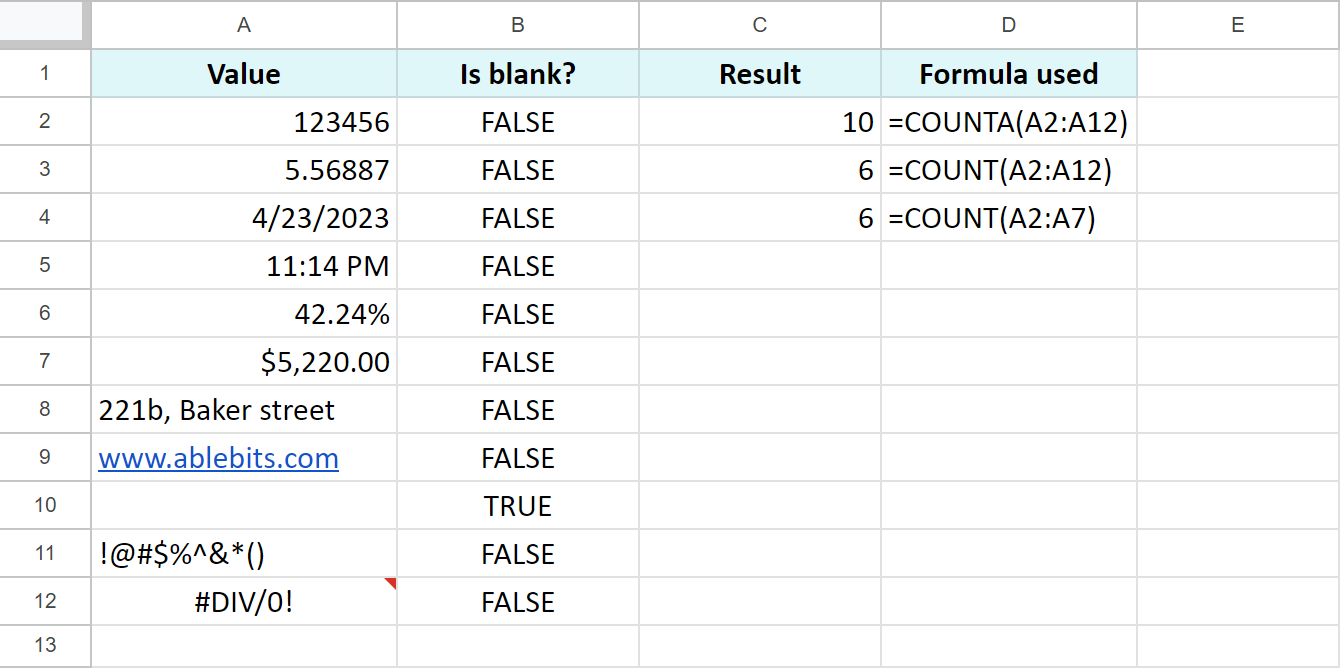
Since date and time are stored and counted as numbers in Google Sheets, both COUNT and COUNTA process A4 and A5.

A10 is completely empty — thus, ignored by both functions.

Other cells were counted by Google Sheets COUNTA:

=COUNTA(A2:A12)

Both formulas with COUNT return the same result because A8:A12 doesn't contain numeric values.

A8 on its turn has a number stored as text which wasn't processed by Google Sheets COUNT.

The error message in A12 is entered as text and considered by COUNTA only.

How to use Google Sheets COUNT and COUNTA — examples included

Let's take a closer look at how the COUNT function is used in a Google spreadsheet and how you can benefit from using it in Sheets.

Suppose you have a list of students' grades. Here are the ways COUNT can help:

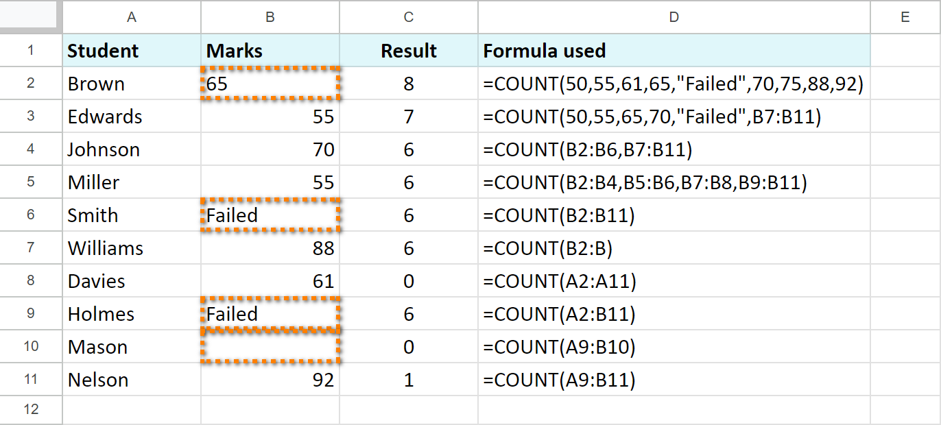
Look, there are different formulas with COUNT in column C.

Since column A contains surnames, COUNT ignores that whole column. But what about cells B2, B6, B9, and B10? B2 has a number formatted as text; B6 and B9 contain pure text; B10 is completely empty.

Another cell to bring your attention to is B7. It has the following formula:

=COUNT(B2:B)

Notice that the range starts from B2 and includes all other cells of this column. This is a very useful method when you often need to add new data to the column but want to avoid changing the range of the formula every time.

Now, how will Google Sheets COUNTA work with the same data?

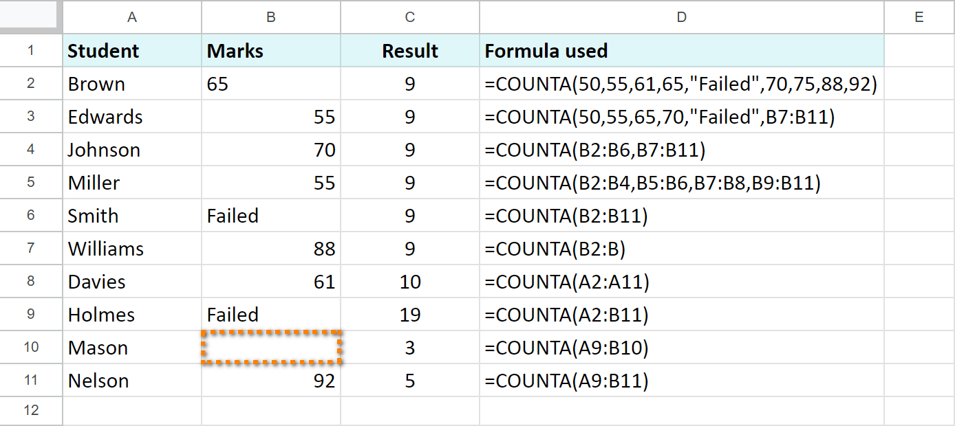
As you can see and compare, the results differ. This function ignores only one cell — the completely empty B10. Thus, bear in mind that COUNTA includes textual values as well as numeric ones.

Here's another example of using COUNT to find an average sum spent on products:

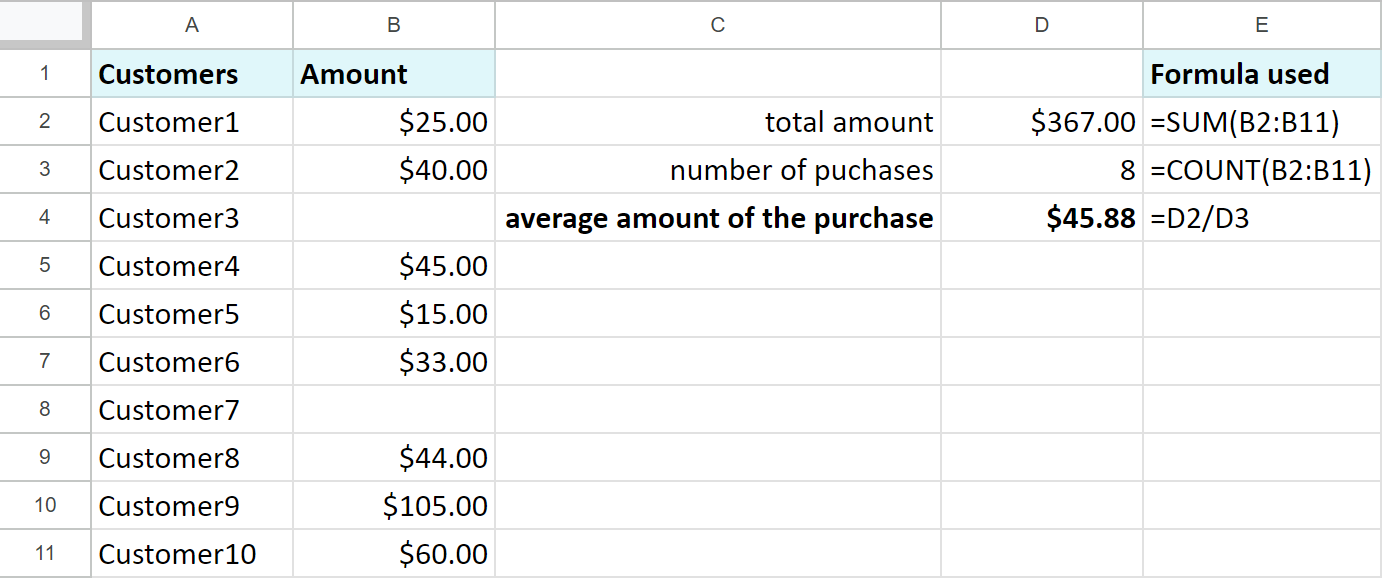
The customers who haven't bought anything are not considered for the results.

One more peculiar thing regarding COUNT in Google Sheets concerns merged cells. There is a rule that COUNT and COUNTA follow to avoid double counting.

When the range for counting contains merged cells, they will be treated by both functions only if the upper-left cell falls within the counted range.

For example, I merge B6:C6 and B9:C9 and count column B. My formula below will count 65, 55, 70, 55, 81, 88, 61, 92:

=COUNT(B2:B)

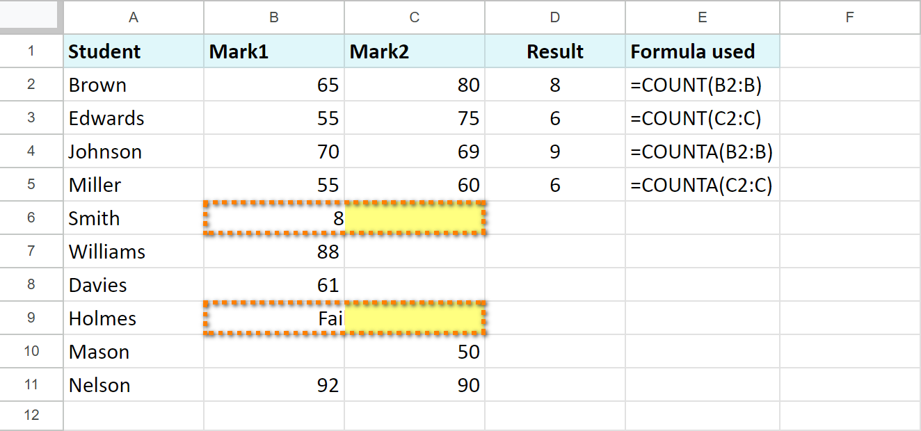
But with a slightly different range, the formula returns another result. It will work only with 80, 75, 69, 60, 50, 90:

=COUNT(C2:C)

The left parts of the merged cells are excluded from this range, therefore are not considered by COUNT.

COUNTA works in a similar way.

1. =COUNTA(B2:B) counts the following: 65, 55, 70, 55, 81, 88, 61, "Failed", 92. Just like with COUNT, empty B10 is ignored.
2. =COUNTA(C2:C) works with 80, 75, 69, 60, 50, 90. Empty C7 and C8, as in the case with COUNT, are ignored. C6 and C9 are omitted from the result since the range doesn't include the leftmost cells B6 and B9.

Count uniques in Google Sheets

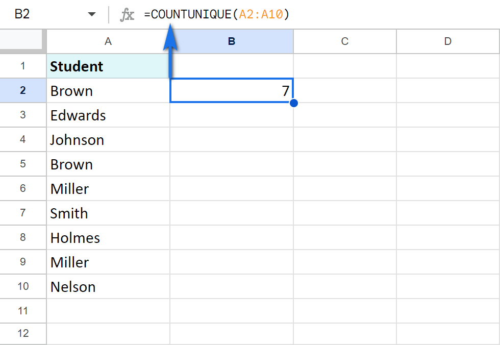
If you'd rather count only unique values in the range, you'd better use the COUNTUNIQUE function. It requires literally one argument that can be repeated: a range or a value to process.

The formulas in spreadsheets will look as plain as this:

=COUNTUNIQUE(A2:A10)

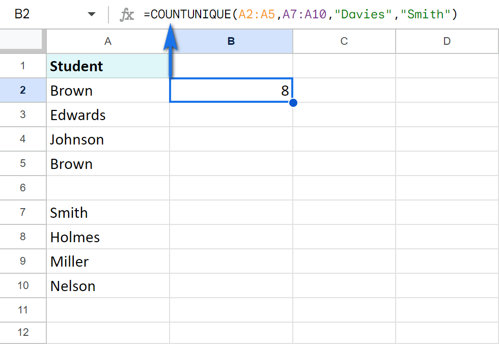
You can also enter multiple ranges and even records themselves directly to the formula:

=COUNTUNIQUE(A2:A5,A7:A10,"Davies","Smith")

Count with multiple criteria — COUNTIF in Google Sheets

In case the standard count is not enough and you need to count only specific values based on some conditions, there is another special function for that — COUNTIF. All its arguments, usage, and examples are covered in another special blog post.

To count & highlight duplicates in Google Sheets, visit this article instead.