It often happens that we need to attach a price to a certain currency. At the same time, the item may be sold in various currencies. Google Sheets contains an extremely convenient tool for currency conversion that you won't find in other programs.
I'm speaking about the GOOGLEFINANCE function. It retrieves current or archival financial information from Google Finance. And today we'll examine the function together.
How to use GOOGLEFINANCE to get current currency exchange rates
Even though GOOGLEFINANCE is capable of many things, we're interested in its ability to fetch currency exchange rates. The syntax of the function is as follows:

Note. The arguments of the function CURRENCY:<from currency symbol><to currency symbol> must be text strings.
For example, to get the current USD to EUR exchange rate, you can use the formula below:
=GOOGLEFINANCE("CURRENCY:USDEUR")
The same can be applied to convert $ to £:
=GOOGLEFINANCE("CURRENCY:USDGBP")
And US dollar to Japanese yen:
=GOOGLEFINANCE("CURRENCY:USDJPY")
To convert currencies even easier, just replace the text in the formulas with cell references:

Here B3 contains the formula that combines two currency names in A1 and A3:
=GOOGLEFINANCE("CURRENCY:"&$A$1&A3)
Tip. You will find a full list of all currency codes including few cryptocurrencies below.
GOOGLEFINANCE to get currency exchange rates over any period of time
We can use the GOOGLEFINANCE function to see how the currency exchange rates have changed over a specified period of time or for the last N days.
Exchange rates over a specified period of time
To pull exchange rates over some period of time, you need to extend your GOOGLEFINANCE function with additional optional arguments:
- attribute (optional) - use "price" to get real time currency exchange rates (with a short delay up to 20 minutes)
Tip. See a full list of available attributes here.
- start_date, end_date (optional) - your period of interest. Use the DATE function in these arguments.
- interval (optional) - how often you wish to pull the data. It can be "DAILY" or "WEEKLY", or in numbers - 1 for daily, 7 for weekly.
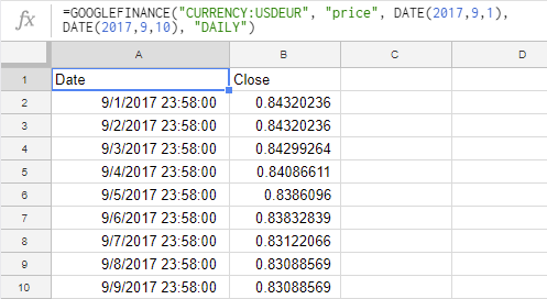
Here's an example of such a formula:
=GOOGLEFINANCE("CURRENCY:USDEUR", "price", DATE(2017,9,1), DATE(2017,9,10), "DAILY")
As a result, we have a table with the rates finalized at the end of the day.

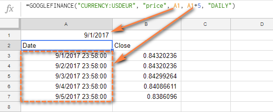
You can use cell references instead of dates to simplify the formula and adjust it in a couple of clicks:
=GOOGLEFINANCE("CURRENCY:USDEUR", "price", A1, A1+5, "DAILY")
A1 is a start date, and we add the needed number of days to it:

Exchange rates for the last N days
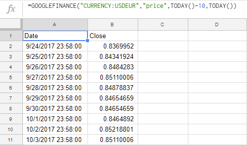
We can also use the GOOGLEFINANCE function to pull the exchange rates for the last N days (10 days in the formula below):
=GOOGLEFINANCE("CURRENCY:USDEUR","price",TODAY()-10,TODAY())

Get exchange rates easier using cell references
One more example of GOOGLEFINANCE in Google Sheets illustrates how you can use cell references in all arguments of the function.
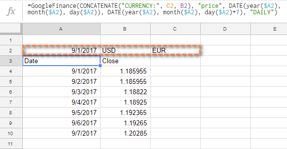
Let's find out the EUR to USD exchange rates over a 7-day period:
=GOOGLEFINANCE(CONCATENATE("CURRENCY:", C2, B2), "price", DATE(year($A2), month($A2), day($A2)), DATE(year($A2), month($A2), day($A2)+7), "DAILY")

The source data - currency codes and start date - are in A2:C2.
To combine a few variables into one, we use the CONCATENATE function instead of a traditional ampersand (&).
The DATE function returns year, month, and day from A2. Then we add 7 days to our start date.
We can always add months as well:
=GOOGLEFINANCE(CONCATENATE("CURRENCY:", C2, B2), "price", DATE(year($A2), month($A2), day($A2)), DATE(year($A2), month($A2)+1, day($A2)+7), "DAILY")
All currency codes for the GOOGLEFINCANCE function
Currency codes consist of ALPHA-2 Code (2-letter country code) and of the first letter of the currency name. For example, the currency code for Canadian dollar is CAD:
CAD = CA (Canada) + D (Dollar)
To use the GOOGLEFINANCE function properly, you need to know currency codes. Below you will get a full list of currencies of the world along with few cryptocurrencies supported by GOOGLEFINANCE.
I hope that this article will help you get the up-to-date information about currency exchange rates and you won't be caught unawares when it comes to working with finances.
Spreadsheet with currency codes
Currency exchange rates for GOOGLEFINANCE (make yourself a copy if you need to edit)
 by
by
57 comments
Houston, we've got a couple of issues!
My Google Sheets don't seem to support this.
Furthermore, it is regrettable that the parameters contain names of fixed currencies. In what sense?
In one cell, I have the base currency, and in another, I have the currency I need to convert. Thus, I require something akin to googlefinance Indian Crypto Coin).
Hello Alisha,
Sorry, it's hard to tell what's going on on your side. For me to be able to help you, please consider sharing an editable copy of your spreadsheet with us (support@apps4gs.com) with your formula and the example of the expected result. I'll look into it and try to help.
Note. We keep that Google account for file sharing only and don't monitor its Inbox. Do not email there. Once you share the file, just confirm by replying to this comment.
Nice Article and Helpful
Hi,
Date time and stock will be entered into column A1 and B1. I want to get the price of the A1,B1 in C1, and have that number no longer update. In D I want the price to be tracked, like Google Finance normally functions in the same row.
That's the goal. Any help would be very much appreciated :)
Hi Fahad,
Please consider sharing an editable copy of your spreadsheet with us (support@apps4gs.com) with 2 sheets: (1) a copy of your source data (2) the result you expect to get. I kindly ask you to shorten the tables to 10-20 rows.
Note. We keep that Google account for file sharing only and don't monitor its Inbox. Please do not email there. Once you share the file, just confirm by replying to this comment.
I'll look into it and try to help.
Hi There,
I am trying to convert my Excel file into a Google Sheet.
In Excel, I can easily obtain the high52 and low52 for an exchange rate USDEUR.
However, I can't get it right in Google Sheet.
Can anyone explain why this works - =GOOGLEFINANCE(A2,"high52") with A2=GOOG but the same with A2=USDEUR doesn't?
Hello!
I have to convert lots of rows of USD to CDN for the specific dates on my spreadsheet.
So...
Date - B2,B3,B4...etc
USD - I2, I3,I4... (known)
CAD - J2,J3,J4... (unknown)
What is the formula to convert USD in column I to CAD in column J with the exchange rate for that date in column B?
Thanks in advance
Hello Adam,
You may try solutions offered some time ago to Brian, please see these comments below.
Hi guys,
I'm trying to write a prediction formula for the USD/TRY. I'm trying to do a budget for FY22. I know noone can not predict it but maybe someone used a formula which makes the prediction more stable.
Did you ever try such kind of a formula for any kind of currency vs ?
Hi Emrah,
No, sorry, we've never tried that. You may try to find a solution here – an overview of Google Apps Script with a lot of helpful content and links: https://developers.google.com/apps-script/overview
Or in Google Sheets Community: https://support.google.com/docs/threads?hl=en&thread_filter=(category:docs_sheets)
how do i get the changepct for currency?
Hello Stephon,
"changepct" doesn't work for currencies at the moment I'm afraid. You can try solutions similar to this one: https://www.reddit.com/r/googlesheets/comments/nbausy/change_percent_for_bitcoin_price/
Hi,
I am unable to get the BTC Close price Only on a certain date, would someone be able to help with the formula for that please.
Regards
Hi Shashankraj,
Please specify the formula that doesn't work for you.
You haven't included cryptocurrencies such as Bitcoin (BTC) in your full list
Hello Olly,
That's a fair point :) GoogleFinance supports only few cryptocurrencies but, nevertheless, I've just added them to the list. Thank you!
I don't need to list the exchange rate. I would like to simply grab it to use a multiplier.
For example:
Column A: Date
Column B: price in CNY
Column C: price in EUR
I want to use a formula in Column C to convert the amount in B using the rate from the date in A.
Is this possible using the googlefinance functionality?
Thanks for all your help.
Hello Brian,
you can use GOOGLEFINANCE straight in the formula as a multiplier only if you don't reference any date:
=B2*GOOGLEFINANCE(CONCATENATE("CURRENCY:",B1,C1))
As soon as you add the date attribute, the formula will fetch historic data in two columns: date and rate. Only then you'll be able to reference a column with the rate in your multiplication.
you can also use something like =average(index(GOOGLEFINANCE(CONCATENATE("CURRENCY:", E3, F$1), "price", B3,1,"DAIlY"),,2)) and it will return the value of the currency exchange rate on date B3
Yes, this works as well, thanks, Eyal!
Natalia can you please explain how this works? Would it be possible to break this down so that I can use it for my own use case?
Hello Laye,
If you're not familiar with other functions used with GOOGLEFINANCE, I'd recommend looking through these articles:
CONCATENATE
INDEX
AVERAGE
Hi, Is it possible to obtain BID and ASK foreign prices with = GOOGLE FINANCE?
Hi Gerardo,
I'm afraid not. You can check a full list of everything you can get with the function (its attributes used for these purposes) here.
Hi, I was wondering if there's any possibility of automating the process - I'm creating a spreadsheet for around 40 currencies and I have a defined period of time (05/31/2017-05/29/2020) but for now I have been just copying and pasting more or less the same formula "GOOGLEFINANCE("CURRENCY:USDAED";"Close"; DATE(2017;5;31); DATE(2020;5;29); "DAILY")" and then I would just change the name of the second currency, but since I have a lot of them it takes quite some time, is there any way to make google sheet just copy and paste the names of the currencies automatically without me having to do it manually?
Hi Alice,
Well, there are lots of currencies and you will still have to say Google which one you need. You can try and enter all currency names in another sheet and reference them in the formula like this:
=GOOGLEFINANCE("CURRENCY:USD"&Sheet2!A2,"Close", DATE(2017,5,31), DATE(2020,5,29), "DAILY")
But since cell references adjust themselves when you copy the formula to other cells, you need to arrange currency names in that second sheets in such a way so when you copy the formula in Sheet1 to, say, C2, C2 in Sheet2 would contain another currency name.
great. thank you.
Hi,
Thanks for the article, i would like to calculate the average exchange rate between two dates with only one formula. Do you know how we could do that ?
Thanks
Hi Jeremy,
Please check out this part of the blog post: Exchange rates over a specified period of time
I'm looking to calculate the average FX rate over the last 365 days, but return a single value vs listing the FX rate for every single day. Is there a way to do that?
Hello Sy,
Please have a look at the following formula example for getting the exchange rate for the last N days: Exchange rates for the last N days
Once you have the formula, paste it in another formula like below to get the average as a single value as well:
=AVERAGE(INDEX(GoogleFinance(YOUR_FORMULA_WITH_EXCHANGE_RATE_OVER_THE_YEAR),,2))
I'm trying to convert many currencies to INR but while the formula encounters INRINR it throws up an error. Can you help me out?
Hello Sumit,
Can you share the exact formula you created? Also, please describe the task in more detail. Do you have a list of all currencies that you're trying to convert including INR?
Hi How do i display the Currency name? eg. for IRR or AUD? in teh column beside the currency symbol?
Hi Michael,
If I'm getting your task correctly and if it's these two currencies only, you can create an IF formula like this:
=IF(ISNUMBER(SEARCH("AUD",A2))=TRUE,"Australian Dollar",IF(ISNUMBER(SEARCH("IRR",A2))=TRUE,"Iranian Rial",""))
If there can be literally any currency, you should use Scripts. Here's an overview of Google Apps Script with a lot of helpful content and links.
I saw your response about getting currency full-names in Google Sheets. It seems to be impossible to do via GOOGLEFINANCE. For stocks (e.g. Tesla), one can just do "GOOGLEFINANCE("TSLA", "name"). However, for currencies, there is no way to retrieve the full name. Also, Google AppScripts does not support any GoogleFinance functionality, so the GoogleFinance APIs can only be used from within Google Sheets itself
Thank you for pointing that out, Curious.
In this case, I'm afraid, some other function, like IF in my example, is the easiest workaround since GOOGLEFINANCE doesn't return full currency names. Alternatively, one could learn more about Google Data Studio or even other finance APIs, like Yahoo Finance API. As for the latter, I would look through its documentation first. We don't use it and cannot guarantee anything, it's just an alternative the Web offers. If you have any other ways in mind, feel free to share!
Hello, I have a list with three columns, base currency, foreign currency and date, the formula =GOOGLEFINANCE("currency:"&E2&F2,"price",G2) works, but only with one row, I am trying to expand it to use it for all rows, but I get an error since the result is not just a cell but a table with a row of titles (date and close) and a row of values. Is there any workaround for this?
Hello Christina,
I'm afraid such array formulas like GoogleFinance cannot be expanded if the range is filled with something else, for example, other formulas.
Formula works perfectly but when I convert EUR to PLN it shows 69.36530277!
It's exactly correct but I don't want to have so many number on a single cell. Is there a possibility to round the number to 67 for example?
Hello Beka,
You can decrease the number of decimal places using the corresponding tool on the Google Sheets toolbar. The screenshot here shows where to find it.
Or you can wrap your GoogleFincance in the ROUND function.
Hi, I copy and paste =GOOGLEFINANCE("CURRENCY:USDEUR","price",TODAY()-10,TODAY()) and answer is #ERROR! . Why? What Did I Do Wrong? 10 in TODAY()-10 didnt light.
Hi Martin,
Go to File > Spreadsheet settings and check your locale. It may not recognise a comma as a separator and require a different one. You will see which one you need in a formula example when you click the formula in the formula bar.
I use paypal is it possible to change the formula to take into account their commission structure. Apologies if this is too easy a question. For Example If I were to change $1000 it is £767.995 using your formula but the actual exchange using paypal is £802.
Thank you
Hello Andrew,
I'm afraid it's impossible since the function is designed by Google in a way to fetch data from Google Finance only.