Learn how to quickly highlight the entire row based on a single cell's value in Excel. Tips and formula examples for number and text values.
Last week we discussed how to change the background color of a cell based on its value. In this article you will learn how to highlight entire rows in Excel based on a value of one cell, and also find a few tips and formula examples that will work with numerical and text cell values.
How to change a row color based on a number in a single cell
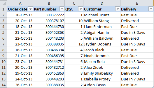
Say, you have a table of your company orders like this:

You may want to shade the rows in different colors based on the cell value in the Qty. column to see the most important orders at a glance. This can be easily done using Excel Conditional Formatting.
- Start with selecting the cells the background color of which you want to change.
- Create a new formatting rule by clicking Conditional Formatting > New Rule… on the Home tab.

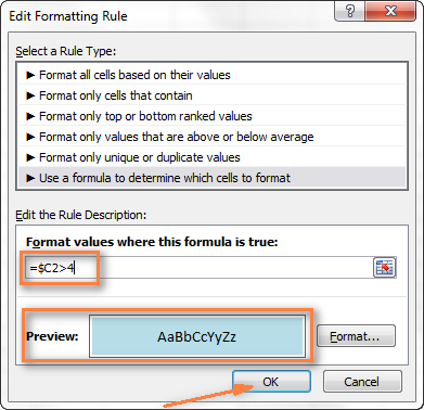
- In the "New Formatting Rule" dialog window that opens, choose the option "Use a formula to determine which cells to format" and enter the following formula in the "Format values where this formula is true" field to highlight orders with Qty. larger than 4:
=$C2>4
And naturally, you can use the less than (<) and equal to (=) operators to find and highlight rows that have Qty. smaller than 4 or equal to 4:
=$C2<4=$C2=4Also, pay attention to the dollar sign $ before the cell's address - it is needed to keep the column letter the same when the formula gets copied across the row. Actually, it is what does the trick and applies formatting to the whole row based on a value in a given cell.
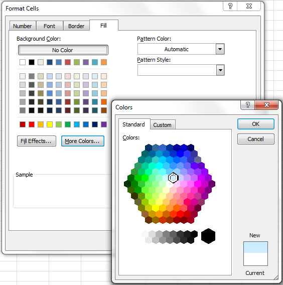
- Click the "Format…" button and switch to Fill tab to choose the background color. If the default colors do not suffice, click the "More Colors…" button to pick the one to your liking, and then click OK twice.

You can also use any other formatting options, such as the font color or cells border on the other tabs of the Format Cells dialog.
- The preview of your formatting rule will look similar to this:

- If this is how you wanted it and you are happy with the color, click OK to see your new formatting in effect.
Now, if the value in the Qty. column is greater than 4, the entire rows in your Excel table will turn blue.

As you can see, changing the row's color based on a number in a single cell is pretty easy in Excel. Further on, you will find more formula examples and a couple of tips for more complex scenarios.
How to apply several rules with the priority you need
In the previous example, you may want to highlight the rows with different values in the Qty. column in different colors. For example, you can add a rule to shade the rows with quantity 10 or greater. In this case, use this formula:
=$C2>9
After your second formatting rule is created, set the rules priority so that both of your rules will work.
- On the Home tab, in the Styles group, click Conditional Formatting > Manage Rules… .
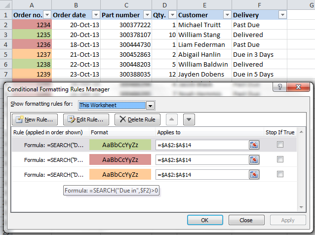
- Choose "This worksheet" in the "Show formatting rules for" field. If you want to manage the rules that apply to your current selection only, choose "Current Selection".
- Select the formatting rule you want to be applied first and move it to the top of the list using the arrows. The result should resemble this:

Click the OK button and the corresponding rows will immediately change their background color based on the cell values that you specified in both formulas.

How to change a row color based on a text value in a cell
In our sample table, to make follow-up on orders easier, you can shade the rows based on the values in the Delivery column, so that:
- If an order is "Due in X Days", the background color of such rows will turn orange;
- If an item is "Delivered", the entire row will be colored in green;
- If an order is "Past Due", the row will turn red.
Naturally, the row color will change if the order status gets updated.
While the formula from our first example could work for "Delivered" and "Past Due"(=$E2="Delivered" and =$E2="Past Due"), the task sounds a bit trickier for "Due in…" orders. As you see, different orders are due in 1, 3, 5 or more days and the above formula won't work because it is purposed for exact match.
In this case, you'd better use the SEARCH function that works for the partial match as well:
=SEARCH("Due in", $E2)>0
In the formula, E2 is the address of the cell that you want to base your formatting on, the dollar sign ($) is used to lock the column coordinate, and >0 means that the formatting will be applied if the specified text ("Due in" in our case) is found in any position in the cell.
Create three such rules following the steps from the first example, and you will have the below table, as the result:

Highlight row if cell starts with specific text
Using >0 in the above formula means that the row will be colored no matter where the specified text is located in the key cell. For example, the Delivery column (F) may contain the text "Urgent, Due in 6 Hours", and this row will be colored as well.
To change the row color when the key cell starts with a particular value, use =1 in the formula, e.g.:
=SEARCH("Due in", $E2)=1
in this case, the row will only be highlighted if the specified text is found in the first position in the cell.
For this conditional formatting rule to work correctly, make sure there are no leading spaces in the key column, otherwise you might rack your brain trying to figure out why the formula does not work :) You can use this free tool to find and remove leading and trailing spaces in your worksheets - Trim Spaces tool for Excel.
How to change a cell's color based on a value of another cell
In fact, this is simply a variation of changing the background color of a row case. But instead of the whole table, you select a column or a range where you want to highlight rows and use the formulas described above.
For example, we could create three such rules to shade only the cells in the "Order number" column based on another cell value (values in the Delivery column).

Highlight rows based on several conditions
If you want to shade the rows in the same color based on several values, then instead of creating several formatting rules you can use the OR or AND functions to set several conditions.
For example, we can color the orders due in 1 and 3 days in the reddish color, and those that are due in 5 and 7 days in the yellow color. The formulas are as follow:
=OR($F2="Due in 1 Days", $F2="Due in 3 Days")
=OR($F2="Due in 5 Days", $F2="Due in 7 Days")

And you can use the AND function, say, to change the background color of rows with Qty. equal to or greater than 5 and equal to or less than 10:
=AND($D2>=5, $D2<=10)

Naturally, you are not limited to using only 2 conditions in such formulas, you are free to use as many as you need. For example:
=OR($F2="Due in 1 Days", $F2="Due in 3 Days", $F2="Due in 5 Days")
Tip: Now that you know how to color cells to differentiate between various types of values, you may want to know how many cells are highlighted in a certain color and calculate the sum of values in those cells. The good news is that you can automate this too and you will find the solution in this article: How to count, sum and filter cells by color in Excel.
These are only a few of many possible ways to zebra stripe your Excel worksheets based on a cell's value that will respond to change of data in that cell. If you need something different for your data set, drop us a comment and we will try to figure this out.
 by
by
102 comments
This was enormously helpful. Very clear and covered all the bases.
I am trying to set it up so that when I input text into a certain column it changes the whole row to a certain color. For example, I have 2 columns that i need this for. One column is "APPROVED" and the other is "DELIVERED". For the APPROVED column when i input the text for who approved it (name) and the date i need that whole row to change to a certain color. For the DELIVERED column when i input the date i need it to change to a different color than the APPROVED column. I hope that makes sense.
Hi! All the information you need to change the color of a row by condition is in the article above. To change the color of a cell by condition, use these recommendations: Excel conditional formatting formulas based on another cell. Create the first conditional formatting rule for a row and the second rule for a cell.
Hello,
I would like the row in my spreadsheet to change colors once a date has been added to the "Date Complete" column. I have tried using =CELL("format",$D2)="D1" type formula, but have found that since I have formatted the cells in column D, the entire spreadsheet changes color. How can I get the row to change color if there is a date in the column, and not change color if there is no date in the column?
Hello! Try adding a second condition: the cell must contain a number. Use ISNUMBER function.
=(LEFT(CELL("format",$D2),1)="D")*ISNUMBER(D2)
I'm trying to have rows turn grey if the customer enquiring is outside of our coverage area (multiple post codes) so can it do it saying if the cell doesn't contain NR or IP it turns the whole row grey?
Hi! Please try the following conditional formatting formula:
=OR(ISNUMBER(SEARCH("NR",A1)),ISNUMBER(SEARCH("IP",A1)))
For more information, please read: How to find substring in Excel
Hello!
I am trying to create a Gantt style chart to track the progress of some upcoming projects and it has been requested that the actual completion date be a different color based on where it falls in the 'allowable timeframe'.
The below formula adds a corresponding filled cell in the calendar side but I am only able to figure out how to do it in one color. I would like to be able to do it in Green, Amber and Red based on how it falls in comparison to the completed date.
=AND(Actual_Completion_Date4>=M$9,Actual_Completion_Date4<N$9)
I have scoured online and would consider myself to have a pretty decent knowledge of Excel, I am coming up blank on this solution. I am not opposed to have multiple formulas in order to get the different colors.
ANY assistance you may be able to provide would be greatly appreciated!
Hello! If I understand the question correctly, you can create a conditional formatting formula for each color. For more information, please read: Excel conditional formatting formulas based on another cell.
On the Spreadsheet I'm making I'm trying to make an entire row change based on whether one cell says "Resolved" or "Not Resolved", I have used the Formula described above, =$B2="Resolved" and =$B2="Not Resolved" Which then Applies to =$A$2:$J$2 but only the cell where the text is Written is colored the rest stay blank
Hi!
I have not been able to replicate your problem. Apply the =$B2="Resolved" rule to the range =$A$2:$J$2 or =$A$2:$J$10
How would I add a color to a portion of a row based upon whether there a cell has information in it or not?
What I'm trying to do is grey out a row if no info has been added to specific cell. Cell 3C has dates in it, but not all rows have dates in the C column. If 3C had no data, I'd like the whole row from 3A-3G to change to grey so it is readily apparent that that line has no information about it. Do you have a suggestion as to how I'd write the formula?
Hi!
Have you tried the ways described in this blog post? The tutorial above contains answers to your question.
For example -
=ISBLANK($C1)
How do you highlight a row just based on a particular cell having text in it? I have a spreadsheet that I want the row to highlight once a date is entered into a cell in column D. I do not know how to make a formula for that.
Hi!
Please re-read the article above, it covers your case completely.
Something like =$D1:$D9999="TEXT" should work for what you are looking for. You can use whatever start/end range for Column D you need and enter the desired text in quotes.
Excellent help page. Thank you.
Hello,
Is it possible to create a formula to number cells, but only the ones, which have one color (e.g. only white ones)?
+ make formula automatically 'refresh' when we decide to change the color of one or two more rows?
KR,
Natalia
Hello!
You can get the cell color in Excel using the user-defined function GetCellColor.
To numbering cells with a specific color in column A, you can use something like this formula starting from cell B2
=IF(COUNT($B$1:B1)=SUM(--("#"&DEC2HEX(GetCellColor($A$2:A2))="#FFFFFF")), "", SUM(--("#"&DEC2HEX(GetCellColor($A$2:A2))="#FFFFFF")))
I hope it’ll be helpful.
Hello There,
I own a food product business. I Have a worksheet where I keep track of deliveries. In the worksheet, against each item, I record Delivery Status(Column K) and Payment Status (Column L). My requirement is two fold.
Rule 1. When Item is delivered, but payment is yet to be received from customer, I want the row colour to change to yellow based on the text "y" in Column K. In this case, corresponding cell in Column K is Blank.
Rule 2. When Payment is received from customer, , I want the row colour to change to green based on the text "y" in Column L. In this case, Column L as well as Column L contain the text "y".
Rule 2 should be applied by overpowering Rule 1.
I am able to set up the rules individually, but I am not yet able to make rule 2 being able to overpower rule 1.
Thanks in advance for your advice.
Regards,
Rucha Mulay
Hello!
Create two conditional formatting rules. Then use the instructions on how to apply multiple conditional formatting rules to a single Excel table.
I hope my advice will help you solve your task.
I want to use conditional format to set the background color for each cell in the B column based on the data in the O Column.
My formula: Formula=$O$2="Cancelled" Format (black color) Applies to =$B$2
Formula =$O$2="Delivered" Format Blue color Applies to $B$2.
I want to be able to select all the cells in Column O and Column B and have the colors change. But this doesn't work. I have to set the 5 different options and type them for every cell.
Hi!
You can only set one format and one color per conditional formatting rule.
You wrote: "In the formula, E2 is the address of the cell that you want to base your formatting on, the dollar sign ($) is used to apply the formula to the entire row..."
This is not entirely correct. Dollar sign is used to turn a relative cell address into an absolute address. The formula for the whole range is based on the formula for the top-left cell and is modified behind the scenes for each cell. Dollar sign anchors the reference to the cell in a specific column and/or row. In this case $E2 means that all cells in the second row will use the value of E2, but cells in row 3 will use the value of cell E3 because column E is locked, but row isn't and moves down. You can test this by changing the cell reference to $E$2. Now all the cells in all rows will be formatted based on the value of E2.
There are 4 possible combinations for a cell reference: E2 (relative address), $E2 (absolute column, relative row), E$2 (relative column, absolute row), and $E$2 (absolute address).
One example: say you have a formula in A1 that says: =D1
If you than copy that formula down into B2 (changing both column and row for demonstration), you can get 4 different results depending on the type of cell address used:
=D1 -> =E2 (B2 is 1 column to the right and 1 row down from A1, and so the target cell also moves the same distance from D1 to E2)
=$D1 -> $D2
=D$1 -> E$1
=$D$1 -> $D$1
Hope this helps :)
Hi Zoran,
Good point! I reworded that sentence.
Hi Svetlana and or Alexander,
I would like to add additional formatting/several rules to a current rule. At the moment I have a current formula for the "top 3 running in cells N2 to N20. It's currently work fine.
My issue that there is other information that I would like to colour in columns L and M that would be associated with the top 3 highlighted cells in N.
Do does one do this? Can it be done?
Hello!
I think you need to add some more conditional formatting rules.
Perhaps this instruction will be useful to you - Apply several conditional formatting rules to one cell and Formulas for conditional formatting based on another cell value.
If this is not what you wanted, please describe the problem in more detail.
Hi,
I want to change cell value based on color and the option available in conditional formatting is in reverse way. Can you suggest.
Thank you.
Hi,
If I understand your task correctly, pay attention to the following paragraph of the article above — "How to apply several rules with the priority you need"
I am using the formula below to try and format rows of data if the number in column C happens to also be in column A of Sheet 1. However, it's only highlighting the first row that meets that condition. All of the other rows that meet the condition are not changing color. Any suggestions?
=$C2=Sheet1!$A:$A
Hello!
If I got you right, the formula below will help you with your task:
=MATCH($C2,Sheet1!$A$1:$A$100,0)
You can learn more about MATCH function in Excel in this article on our blog.
HI there,
I have an excel sheet with columns and want to add another which will have date of expiry in them. I would like that these dates are changed automatically when we get to a month before expiry date to amber and red once its past the date, how can I do this???
Hello!
Please check out the following article on our blog, it’ll be sure to help you with your task: How to conditionally format dates and time in Excel.
I cannot get a pivot table based upon time to conditional format. I have reformatted the numbers to be "general", Time, Custom (mm:ss), text and nothing works. When I use a formula that is built-in, such as "higher than", it highlights the whole column, not distinguishing between values.
Excel 16 Conditional Formatting of time within pivot tables is really difficult!
Hello!
Please have a look at this article — Excel conditional formatting for dates & time.
Hope you’ll find this information helpful.
I have excel sheet and one column I have renewal date. I want to highlight this row before one month
So I can I use this conditional formatting
Please revert on my email
Hello!
Read how to highlight dates within a date range.
Hope you’ll find this information helpful.
How to I apply a color to a single text in a row in excel?
For example: Miniature doll clothing, dress, size 1
I want the no. 1 in red on various rows.
Then, let's say the rest of my 20 rows, the size is size 2, so I want the no. 2 in green
What formula do I use and how?
Thanks
Hello!
I hope you have studied the recommendations in the above tutorial.
Use conditional formatting with a formula. Set the text color to red when this condition is met:
=NOT(ISERROR(SEARCH("1",A1,1)))
For green, use the formula
=NOT(ISERROR(SEARCH("2",A1,1)))
I hope it’ll be helpful.