If you don't want to get lost in all the charts in your Excel worksheet, then spend some minutes to read this article and learn how to add a chart title in Excel 2013 and have it dynamically updated. I'll also show you how to add descriptive titles to the axes or remove a chart or axis title from a chart. There's nothing to it! :)
You have to work a lot in Excel, make thousands of calculations and organize your data using different tables and charts. Your mind starts spinning when you see these yards of facts and figures. No doubt that graphical data are much easier to understand.
The problem is that when you create a basic chart in Excel 2013/2010, a title is not added to it by default. You have to add it manually. If you have just one chart in the worksheet you don't have to pay attention to the absence of the title. But your chart will look by far more attractive with it. Once several diagrams appear in your worksheet you may tie yourself up in a knot.
Add a chart title
Here's a very simple example how to insert a chart title in Excel 2013. This technique works in any Excel version for all chart types.
- Click anywhere in the chart to which you want to add a title.
- Once you select the chart, the CHART TOOLS will appear in the main toolbar. You can see them only if your chart is selected (it has a shaded outline).
In Excel 2013 the CHART TOOLS include 2 tabs: DESIGN and FORMAT.

- Click on the DESIGN tab.
- Open the drop-down menu named Add Chart Element in the Chart Layouts group.
If you work in Excel 2010, go to the Labels group on the Layout tab. - Choose 'Chart Title' and the position where you want your title to display.
You can place the title above the graphical image (it will resize the chart a little bit) or you can choose the Centered Overlay option and place the title right up on the chart and it will not resize it.

- Click inside the title box.
- Highlight the words 'Chart Title' and start typing the desired name for your chart.
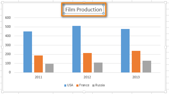
Now it is clear what the chart shows, isn't it?
Format a chart title
- If you go to DESIGN -> Add Chart Element -> Chart Title again and choose 'More Title Options' at the bottom of the drop-down menu, you'll be able to format your chart title.
You'll see the following sidebar to the right of the worksheet.
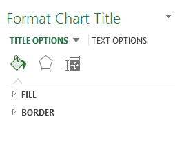
In Excel 2010 you'll find 'More Title Options' at the bottom of the Chart Title drop-down menu in the Labels group on the Layout tab.
Another way to display the Format Chart Title sidebar is just to right-click on the title box and choose 'Format Chart Title' as on the screenshot below.
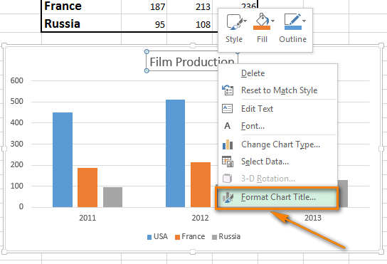
Now you can add a border, fill color or apply 3-D format to the title or change its alignment.
- Right-click on the title box and choose the Font option or use the formatting buttons on the Ribbon (HOME tab, Font group) to format the text. In both cases the following window will display.
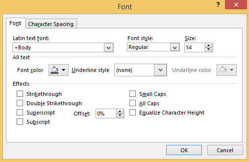
Now you can change the font style, size or color of the title; add different effects to the text; modify character spacing.
Make a dynamic chart title
The time has come for automating the chart title. The solution is quite simple - you need to link the chart title to a cell with a formula.
- Click on the chart title.
- Type the equal sign (=) in the Formula bar.
When you type in the equal sign, please, make sure that it is in the Formula bar, not in the title box. - Click on the cell that you want to link to the chart title.
Note: The cell should have the text that you'd like to be your chart title (as cell B2 in the example below). The cell can also contain a formula. The formula result will become your chart title. You can use the formula directly in the title, but it is not convenient for further editing.
After you do that, you'll see the formula reference including the worksheet name and the cell address in the Formula bar.
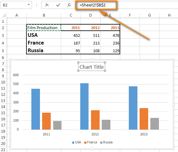
It is very important to type the equal sign (=). If you forget to do it, you will just move to another cell instead of creating the dynamic Excel link.
- Press the Enter button.

So now if I change the text in cell B2, the chart title will be automatically updated.
Add an axis title
A chart has at least 2 axes: the horizontal x-axis (category axis) and the vertical y-axis. 3-D charts also have a depth (series) axis. When the values don't speak for themselves you should include axis titles to clarify what your chart displays.
- Select the chart.
- Navigate to the Chart Layouts group on the DESIGN tab.
- Open the drop-down menu named 'Add Chart Element'.
In Excel 2010 you have to go to the Labels group on the Layout tab and click the Axis Title button.
- From Axis Title options choose the desired axis title position: Primary Horizontal or Primary Vertical.
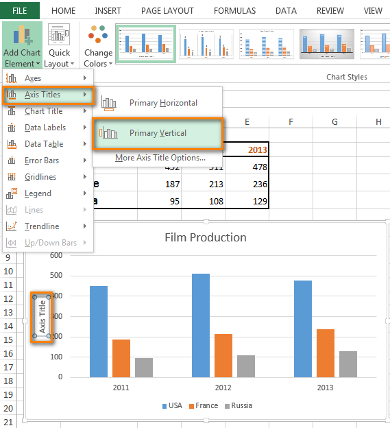
- In the Axis Title text box that appears in the chart, type the text that you want.

If you want to format the axis title, click in the title box, highlight the text that you want to format and go through the same steps as for formatting a chart title. But in the Add Chart Element drop-down menu go to Axis Title -> More Axis Title Options and make the changes you want.
Note: Some chart types (such as radar charts) have axes, but they don't display axis titles. Such chart types as pie and doughnut charts do not have axes at all so they don't display axis titles either. If you switch to another chart type that does not support axis titles, the axis titles will no longer be displayed.
Remove a chart or axis title
Choose one of the solutions below that works best for you to remove a chart or axis title from a chart.
Solution 1
- Click anywhere in the chart.
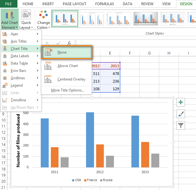
- Open the Add Chart Element drop-down menu in the Chart Layouts group on the DESIGN tab.
- Select the Chart Title option and choose 'None'. Your chart title disappear without a trace.
In Excel 2010 you'll find this option if you click on the Chart Title button in the Labels group on the Layout tab.
Solution 2
To clear off the title in no time, click on the chart title or an axis title and press the Delete button.
You can also right-click on the chart or axis title and choose 'Delete' from the context menu.
Solution 3
If you've just typed in a new title and changed your mind, you can click 'Undo' on the Quick Access Toolbar or press CTRL+Z.
Now you know how to add, format, automate and remove such small but important details as chart and axis titles. Don't forget to use this technique if you want to make a complete and accurate presentation of your work using Excel charts. It's easy and it works!
 by
by
5 comments
I was trying to place a dynamic chart title for a map. I click on the chart title but it will not let me click on the formula bar or at least I can't get the usual response after typing "="?
Any ideas?
Additionally, I can place a dynamic title in the other charts but if I change back to map charts it gives the following message: "Map Charts work best with geographical data..... Check your data and try again." But it's the same data I had when I created the map a step before.
Looks like we have a glitch.
Hi! Unfortunately, I can't create a chart for you in your workbook. Nor can I change the way Excel works.
When I try to do a dynamic title per your example, entering "=A4" in the formual bar (where cell A4 has the text for the title), I get "You can only use external references to worksheets as references in a series formula" (Office 365).
Hi,
To eliminate this error message, type the name of the worksheet before the cell reference (I believe the "!" is a required separator b/w the worksheet name and the cell reference. For example:
=Sheet1!$J$24