Everything you need to know about conditional format for empty cells in Excel
As simple as it may sound, highlighting blank cells with conditional formatting is quite a tricky thing. Basically, it's because a human understanding of empty cells does not always correspond to that of Excel. As a result, blank cells may get formatted when they shouldn't and vice versa. This tutorial will take a close look at various scenarios, share some useful bits on what is happening behind the scenes and show how to make conditional format for blanks work exactly the way you want.
Why does conditional formatting highlight blank cells?
Summary: conditional formatting highlights blank cells because it makes no difference between blanks and zeros. More details follow below.
In the internal Excel system, a blank cell equals a zero value. So, when you create a conditional format for cells less than a certain number, say 20, blank cells get highlighted too (as 0 is less than 20, for empty cells the condition is TRUE).
Another example is highlighting dates less than today. In terms of Excel, any date is an integer greater than zero, meaning an empty cell is always less than today's day, so the condition is satisfied for blanks again.
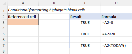
Solution: Make a separate rule to stop conditional formatting if cell is blank or use a formula to ignore blank cells.
Why aren't blank cells highlighted with conditional formatting?
There may be different reasons for blanks not being formatted such as:
- There is the first-in priority rule that stops conditional formatting for empty cells.
- Your formula is not correct.
- Your cells are not absolutely empty.
If your conditional formatting formula uses the ISBLANK function, please be aware that it identifies only truly empty cells, i.e. cells that contain absolutely nothing: no spaces, no tabs, no carriage returns, no empty strings, etc.
For example, if a cell contains a zero-length string ("") returned by some other formula, that cell is not considered as blank:

Solution: If you want to highlight visually empty cells that contain zero-length strings, apply the preset conditional formatting for blanks or create a rule with one of these formulas.
How to highlight blank cells in Excel
Excel conditional formatting has a predefined rule for blanks that makes it really easy to highlight empty cells in any data set:
- Select the range where you wish to highlight empty cells.
- On the Home tab, in the Styles group, click Conditional Formatting > New Rule.
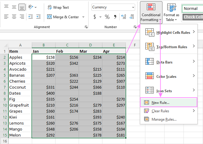
- In the New Formatting Rule dialog box that opens, select the Format only cells that contain rule type, and then choose Blanks from the Format only cells with drop down:

- Click the Format… button.
- In the Format Cells dialog box, switch to the Fill tab, select the desired fill color, and click OK.

- Click OK one more time to close the previous dialog window.
All the blank cells in the selected range will get highlighted:

Tip. To highlight non-empty cells, select Format only cells that contain > No blanks.
Note. The inbuilt conditional formatting for blanks also highlights cells with zero-length strings (""). If you only want to highlight absolutely empty cells, then create a custom rule with the ISBLANK formula as shown in the next example.
Conditional formatting for blank cells with formula
To have more flexibility when highlighting blanks, you can set up your own rule based on a formula. The details steps to create such a rule are here: How to create conditional formatting with formula. Below, we will discuss the formulas themselves
To only highlight truly empty cells that contain absolutely nothing, use the ISBLANK function.
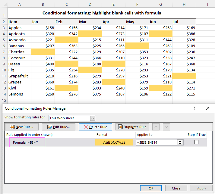
For the below dataset, the formula is:
=ISBLANK(B3)=TRUE
Or simply:
=ISBLANK(B3)
Where B3 is the upper-left cell of the selected range.
Please keep in mind that ISBLANK will return FALSE for cells containing empty strings (""), consequently such cells won't be highlighted. If that behavior is not want you want, then either:
Check for blank cells including zero-length strings:
=B3=""
Or check if the string length is equal to zero:
=LEN(B3)=0
Aside from conditional formatting, you can highlight blank cells in Excel using VBA.
Stop conditional formatting if cell is blank
This example shows how to exclude blank cells from conditional formatting by setting up a special rule for blanks.
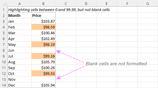
Suppose you used an inbuilt rule to highlight cells between 0 and 99.99. The problem is that empty cells get highlighted too (as you remember, in Excel conditional formatting, a blank cell equals a zero value):

To prevent empty cells from being formatted, do the following:
- Create a new conditional formatting rule for the target cells by clicking Conditional formatting > New Rule > Format only cells that contain > Blanks.
- Click OK without setting any format.

- Open the Rule Manager (Conditional Formatting > Manage Rules), make sure the "Blanks" rule is at the top of the list, and tick the Stop if true check box next to it.
- Click OK to save the changes and close the dialog box.

The result is exactly as you would expect:
Tips:
- You can also exclude blanks by creating a conditional formatting rule with a formula that checks for blank cells and selecting the Stop if true option for it.
- Also, you may be interested to watch a video showing how to apply conditional formatting if another cell is blank.
Conditional formatting formula to ignore blank cells
In case you already use a conditional formatting formula, then you do not really need to make a separate rule for blanks. Instead, you can add one more condition to your existing formula, namely:
- Ignore absolutely empty cells that contain nothing:
NOT(ISBLANK(A1))
- Ignore visually blank cells including empty strings:
A1<>""
Where A1 is the leftmost cell of your selected range.
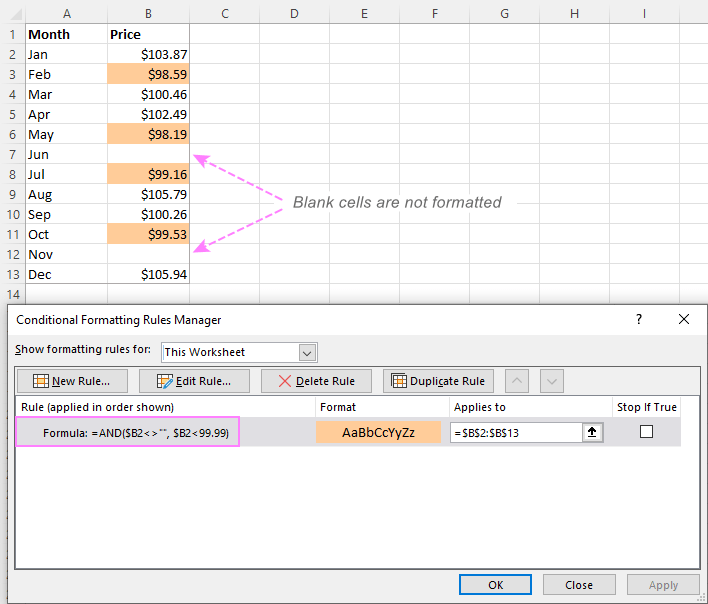
In the dataset below, let's say you wish to highlight values less than 99.99. This can be done by creating a rule with this simple formula:
=$B2<99.99
To highlight values less than 99.99 ignoring empty cells, you can use the AND function with two logical tests:
=AND($B2<>"", $B2<99.99)
=AND(NOT(ISBLANK($B2)), $B2<99.99)
In this particular case, both formulas ignore cells with empty strings, as the second condition (<99.99) is FALSE for such cells.
If cell is blank highlight row
To highlight an entire row if a cell in a specific column is blank, you can use any of the formulas for blank cells. However, there are a couple of tricks you need to know:
- Apply the rule to a whole dataset, not just one column in which you search for blanks.
- In the formula, lock the column coordinate by using a mixed cell reference with an absolute column and relative row.
This might sound complicated on the surface, but it's a lot simpler when we look at an example.
In the sample dataset below, suppose you wish to highlight rows that have an empty cell in column E. To have it done, follow these steps:
- Select your dataset (A3:E15 in this example).
- On the Home tab, click Conditional formatting > New Rule > Use a formula to determine which cells to format.
- In the Format values where this formula is true box, enter one of these formulas:
To highlight absolutely empty cells:
=ISBLANK($E3)To highlight blank cells including empty strings:
=$E3=""Where $E3 is the upper cell in the key column that you want to check for blanks. Please notice that, in both formulas, we lock the column with the $ sign.
- Click the Format button and choose the fill color you want.
- Click OK twice to close both windows.
As a result, conditional formatting highlights a whole row if a cell in a specific column is empty.

Highlight row if cell is not blank
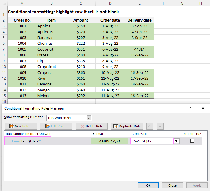
Excel conditional formatting to highlight the row if a cell in a particular column is not blank is done in this way:
- Select your dataset.
- On the Home tab, click Conditional formatting > New Rule > Use a formula to determine which cells to format.
- In the Format values where this formula is true box, enter one of these formulas:
To highlight non-empty cells that contain anything: value, formula, empty string, etc.
=NOT(ISBLANK($E3))To highlight non-blanks excluding cells with empty strings:
=$E3<>""Where $E3 is the topmost cell in the key column that is checked for non-blanks. Again, for the conditional formatting to work correctly, we lock the column with the $ sign.
- Click the Format button, choose your favorite fill color, and then click OK.
As a result, an entire row gets highlighted if a cell in a specified column is not empty.
Excel conditional formatting for zeros but not blanks
By default, Excel conditional formatting does not distinguish between 0 and blank cell, which is really confusing in many situations. To resolve this predicament, there are two possible solutions:
- Create 2 rules: one for the blanks and the other for zero values.
- Create 1 rule that checks both conditions in a single formula.
Make separate rules for blanks and zeros
- First, create a rule to highlight zero values. For this, click Conditional Formatting > New Rule > Format only cells that contain, and then set Cell value equal to 0 like shown on the screenshot below. Click the Format button and select the desired color.
This conditional formatting applies if a cell is blank or zero:

- Make a rule for blanks with no format set. Then, open the Rule Manager, move the "Blanks" rule to the top of the list (if it isn't already there), and tick the Stop if true check box next to it. For the detailed instructions, please see How to stop conditional formatting on blank cells.
As a result, your conditional formatting will include zeros but ignore blanks. As soon as the first condition is met (the cell is empty), the second condition (the cell is zero) is never tested.

Make a single rule to check if cell is zero, not blank
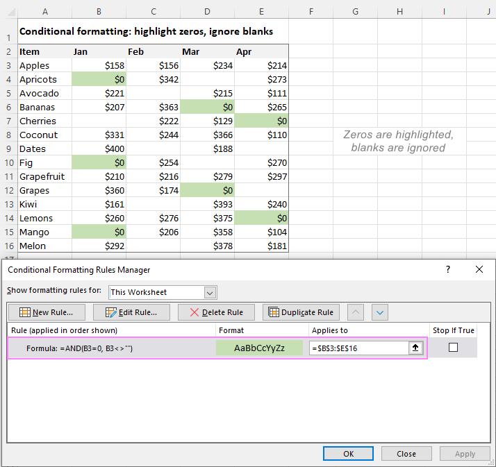
Another way to conditionally format 0's but not blanks is to create a rule with a formula that checks both conditions:
=AND(B3=0, B3<>"")
=AND(B3=0, LEN(B3)>0)
Where B3 is the upper-left cell of the selected range.
The result is exactly the same as with the previous method - conditional formatting highlights zeros but ignores empty cells.
That's how to use conditional format for blank cells. I thank you for reading and look forward to seeing you next week.
Practice workbook for download
Excel conditional formatting for blank cells - examples (.xlsx file)
 by
by
24 comments
Question, doing a comparison between 2 sets of numbers =A5<C5 asking to highlight if A is less than C, why in some cases a zero (0) is entered into the cell with the highlights and other just the highlights?
Hello Richard!
Conditional formatting cannot change the value in a cell. However, you can set your conditional formatting rule to display 0 for empty cells. For more information, please visit: Custom Excel number format.
Hello, I would like an empty cell to automatically be displayed in the same color as the cell above it. How do I do this?
Hi! You can get the cell color code using custom function GetCellColor. For a detailed description and examples, see this article: How to sum and count cells by color in Excel.
However, you can only highlight a cell with the same color as the cell above using a VBA macro.
Hello,
I have data that can be added in column E or F. Sometimes column E&F are both blank, sometimes E only is populated, and sometimes E&F are both populated.
Is there a way to highlight if in any given row E&F are different, but only if both cells are populated?
Hi! To select cells according to your conditions, you can use a conditional formatting formula like this:
=AND(E1<>F1,E1<>"",F1<>"")
Maybe this article will be helpful: Excel conditional formatting formulas based on another cell
How do you set up conditional formatting to highlight all blank cells in a row IF the cell in column A is not blank?
=AND($A2"",ISBLANK(B2:Y2)) is not working.
Hello Abigail!
For the cell range B2:Y30, use the conditional formatting rule
=AND($A1<>"",B1="")
For more information, please visit: Relative and absolute cell references in Excel conditional formatting.
I am trying to adjust some conditional formatting, i'd like to not be able to select a specific option from the drop down menu in column P if column O is blank, but i'm struggling to find the formula to do this, could someone help please?
Hi! You can activate a drop-down list by a condition using VBA. You cannot do it with a formula.
Hi,
Please would anyone be kind to shed light on the following:
I have a series of columns, in which some cells have entry and some not, representing combinations of some sorts.
Is there a way to highlight the columns that have same cells relative to their row filled, in order to spot repeated combination?
Thank you very much.
Hi! If I understand your task correctly, this article may be helpful: How to highlight duplicate cells and rows in Excel. If this does not help, explain the problem in detail.
I am trying to highlight the cell beside a blank cell. Example cell 2a has no information in it so I want to highlight cel 3a for new input of information.
Hi! I can't offer you a formula since cell 2a doesn't exist. Maybe this article will be helpful: Excel conditional formatting formulas based on another cell.
How do i set up conditional formatting to highlight an entire row if 1. a cell in Column N has a number value above 1 and 2. a cell in Column P of the same row is empty. If it wont highlight the entire row, that is fine at least highlight the cell in "N" if the cell in "P" is not blank
Example:
N3 value is greater than 1, P3 is blank- highlight row 3, or at least highlight N3 and P3
N3 value is greater than 1, P3 is not blank- nothing happens.
Hi! Try to use the recommendations described in this article: How to change the row color based on a cell value in Excel.
For the range starting from the first row, this conditional formatting formula is suitable:
=AND($N1>1,ISBLANK($P1))
This is really helpful - Thank you. I'm not great at formulas so still struggling with one aspect. Not sure if it's possible?
Looking to highlight a cell if the value of either of 2 cells in the same row has a number greater than zero in it, and the cell I'm looking to highlight is empty.
In case it's not clear:
QTY of product shipped in O2 = 1
If there is no shipping reference in M2 and/or no invoice # in N2 then the cell with the missing info (either M2 and/or M2) is highlighted.
It's basically a check to ensure that once something has been allocated and marked as shipped, the invoice # and the shipping reference is entered. If not, then the highlighted cell will draw attention to it.
Hope this makes sense....
I'm pretty sure I can do it but not sure the best way
Cheers
Matthew
Hi! To highlight cells in columns M and N using conditional formatting, try this formula:
=AND($O1>0,ISBLANK($M1),ISBLANK($N1))
For more information, please visit: Excel conditional formatting formulas based on another cell.
Hello,
I am looking to color fill cells in a row that is blank with red when there is any text in column A in the row. For example is there is text in A2, I want to highlight all blank cells from B2:I2. I then want to repeat the process for Rows 3 through 18 to follow the same.
Hi! Create a conditional formatting rule for the range B2:I18 with a formula:
=AND($A2<>"",ISBLANK(B2))
For mire information, read: Change the row color based on cell value.
Hi,
I am conditioning a SS to highlight a row in excel based on the Value "T" but it keep highlighting the row under and not the row that contains the "T".
Hi! Use a reference to row 1 in the conditional formatting formula.
How do I change the automatic formatting of placing a "-" (minus sign) in blank cells? I presently am filtering for the minus sign (tens of thousands) and changing to (0) (zero) so that my algorithms work. Thank you.
Hello!
If I understand your task correctly, the following tutorial should help: Display zeros as dashes or blanks.