The tutorial shows how to make custom Data Validation rules in Excel. You will find a few examples of Excel data validation formulas to allow only numbers or text values in specific cells, or only text beginning with specific characters, permit unique data preventing duplicates, and more.
In yesterday's tutorial we started to look at Excel Data Validation - what its purpose is, how it works, and how to use built-in rules to validate data in your worksheets. Today, we are going to take a step further and talk about the nitty-gritty aspects of custom data validation in Excel as well as experiment with a handful of different validation formulas.
How to create custom data validation with formula
Microsoft Excel has several built-in data validation rules for numbers, dates and text, but they cover only the most basic scenarios. If you want to validate cells with your own criteria, create a custom validation rule based on a formula. Here's how:
- Select one or more cells to validate.
- Open the Data Validation dialog box. For this, click the Data Validation button on the Data tab, in the Data Tools group or press the key sequence Alt > D > L (each key is to be pressed separately).
- On the Settings tab of the Data Validation dialog window, select Custom in the Allow box, and enter your data validation formula in the Formula box.
- Click OK.
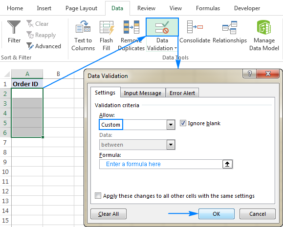
Optionally, you can add a custom input message and Error alert that will show up when the user selects the validated cell or enters invalid data, respectively.
Below you will find a few examples of custom validation rules for different data types.
Note. All Excel data validation rules, built-in and custom, verify only new data that is typed in a cell after creating the rule. Copied data is not validated, nor is the data input in the cell before making the rule. To pin down existing entries that do not meet your data validation criteria, use the Circle Invalid Data feature as shown in How to find invalid data in Excel.
Excel data validation to allow numbers only
Surprisingly, none of the inbuilt Excel data validation rules cater for a very typical situation when you need to restrict users to entering only numbers in specific cells. But this can be easily done with a custom data validation formula based on the ISNUMBER function, like this one:
=ISNUMBER(C2)
Where C2 is the topmost cell of the range you want to validate.
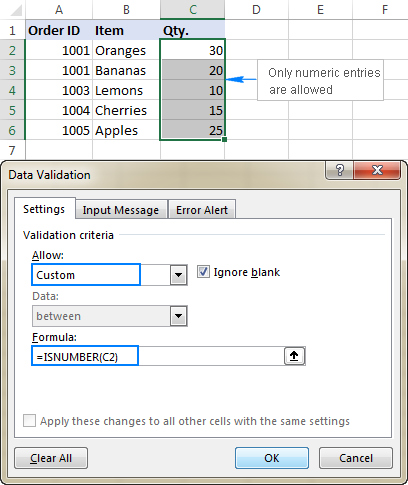
Note. The ISNUMBER function allows any numeric values in validated cells, including integers, decimals, fractions as well as dates and times, which are also numbers in terms of Excel.
Excel data validation to allow text only
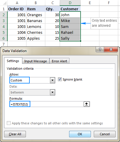
If you are looking for the opposite - to allow only text entries in given range of cells, then build a custom rule with the ISTEXT function, for example:
=ISTEXT(D2)
Where D2 is the uppermost cell of the selected range.
Allow text beginning with specific character(s)
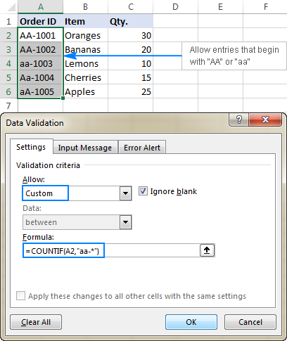
If all values in a certain range should begin with a particular character or substring, then do Excel data validation based on the COUNTIF function with a wildcard character:
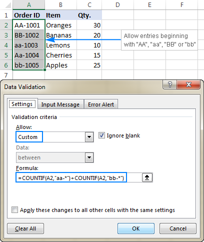
For example, to ensure that all order id's in column A begin with the "AA-", "aa-", "Aa-", or "aA-" prefix (case-insensitive), define a custom rule with this data validation formula:
=COUNTIF(A2,"aa-*")
Validation formula with the OR logic (multiple criteria)
In case there are 2 or more valid prefixes, add up several COUNTIF functions, so that your Excel data validation rule works with the OR logic:
=COUNTIF(A2,"aa-*")+COUNTIF(A2,"bb-*")
Case-sensitive validation formula
If the character case matters, then use EXACT in combination with the LEFT function to create a case-sensitive validation formula for entries beginning with specific text:
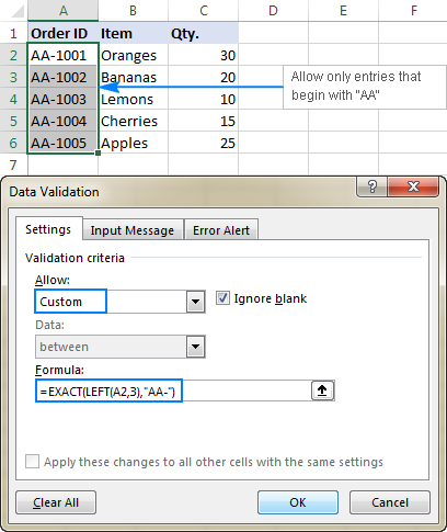
For instance, to allow only those order ids that begin with "AA-" (neither "aa-" nor "Aa-" is allowed), use this formula:
=EXACT(LEFT(A2,3),"AA-")
In the above formula, the LEFT function extracts the first 3 characters from cell A2, and EXACT performs a case-sensitive comparison with the hard-coded substring ("AA-" in this example). If the two substrings match exactly, the formula returns TRUE and the validation passes; otherwise FALSE is returned and the validation fails.
Allow entries containing certain text
To allow entries that contain specific text anywhere in a cell (in the beginning, middle, or end), use the ISNUMBER function in combination with either FIND or SEARCH depending on whether you want case-sensitive or case-insensitive match:
- Case-insensitive validation:
ISNUMBER(SEARCH(text, cell))
- Case-sensitive validation:
ISNUMBER(FIND(text, cell))
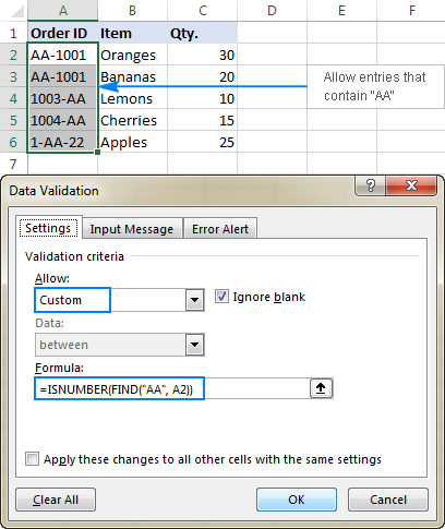
On our sample data set, to permit only entries containing the text "AA" in cells A2:A6, use one of these formulas:
Case-insensitive:
=ISNUMBER(SEARCH("AA", A2))
Case-sensitive:
=ISNUMBER(FIND("AA", A2))
The formulas work with the following logic:
You search the substring "AA" in cell A2 using FIND or SEARCH, and both return a position of the first character in the substring. If the text is not found, an error is returned. For any numeric value returned as the result of search, the ISNUMBER function yields TRUE, and data validation is successful. In case of an error, ISNUMBER returns FALSE, and the entry won't be allowed in a cell.
Data validation to allow only unique entries and disallow duplicates
In situations when a certain column or a range of cell should not contain any duplicates, configure a custom data validation rule to allow only unique entries. For this, we are going to use the classic COUNTIF formula to identify duplicates:
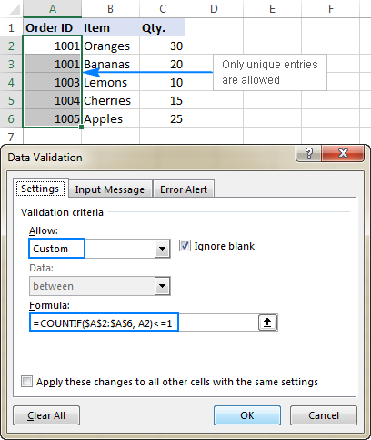
For example, to make sure that only unique order ids are input in cells A2 to A6, create a custom rule with this data validation formula:
=COUNTIF($A$2:$A$6, A2)<=1
When a unique value is entered, the formula returns TRUE and the validation succeeds. If the same value already exists in the specified range (count greater than 1), COUNTIF returns FALSE and the input fails validation.
Please pay attention that we lock the range with absolute cell references (A$2:$A$6) and use a relative reference for the top cell (A2) to get the formula to adjust properly for each cell in the validated range.
Note. This data validation formulas is case-insensitive, it does not distinguish uppercase and lowercase text.
Validation formulas for dates and times
Inbuilt date validation provides quite a lot of predefined criteria to restrict users to entering only dates between the two dates you specify, greater than, less than, or equal to a given date.
If you want more control over data validation in your worksheets, you can replicate the inbuilt functionality with a custom rule or write your own formula that goes beyond the built-in capabilities of Excel data validation.
Allow dates between two dates
To limit the entry to a date within a specified range, you can use either the predefined Date rule with the "between" criteria or make a custom validation rule with this generic formula:
Where:
- cell is the topmost cell in the validated range, and
- start and end dates are valid dates supplied via the DATE function or references to cells containing the dates.
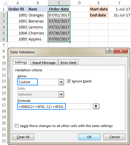
For example, to allow only dates in the month of July of the year 2017, use the following formula:
=AND(C2>=DATE(2017,7,1),C2<=DATE(2017,7,31))
Or, enter the start date and end date in some cells (F1 and F2 in this example), and reference those cells in your formula:
=AND(C2>=$F$1, C2<=$F$2)
Please notice that the boundary dates are locked with absolute cell references.
Allow weekdays or weekends only
To restrict a user to entering only weekdays or weekends, configure a custom validation rule based on the WEEKDAY function.
With the return_type argument set to 2, WEEKDAY returns an integer ranging from 1 (Monday) to 7 (Sunday). So, for weekdays (Mon to Fri) the result of the formula should be less than 6, and for weekends (Sat and Sun) greater than 5.
Allow only workdays:
Allow only weekends:
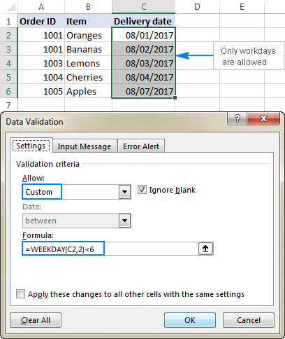
For example, to allow entering only workdays in cells C2:C6, use this formula:
=WEEKDAY(C2,2)<6
Validate dates based on today's date
In many situations, you may want to use today's date as the start date of the allowed date range. To get the current date, use the TODAY function, and then add the desired number of days to it to compute the end date.
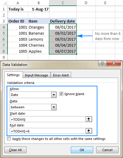
For example, to limit the data entry to 6 days from now (7 days including today), we are going to use the built-in Date rule with the formula-based criteria:
- Select Date in the Allow
- Select between in the Data
- In the Start date box, enter
=TODAY() - In the End date box, enter
=TODAY() + 6
In a similar manner, you can restrict users to entering dates before or after today's date. For this, select either less than or greater than in the Data box, and then enter =TODAY() in the End date or Start date box, respectively.
Validate times based on current time
To validate data based on the current time, use the predefined Time rule with your own data validation formula:
- In the Allow box, select Time.
- In the Data box, pick either less than to allow only times before the current time, or greater than to allow times after the current time.
- In the End time or Start time box (depending on which criteria you selected on the previous step), enter one of the following formulas:
- To validate dates and times based on the current date and time:
=NOW() - To validate times based on the current time:
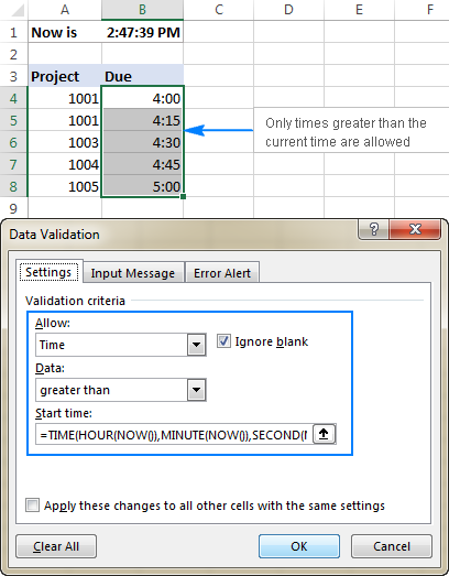
=TIME( HOUR(NOW()), MINUTE(NOW()), SECOND(NOW()))
- To validate dates and times based on the current date and time:
The screenshot below shows a rule that allows only times greater than the current time:
Custom Excel data validation rule not working
If your formula-based data validation rule does not work as expected, there are 3 main points to check:
- Data validation formula is correct
- Validation formula does not refer to an empty cell
- Appropriate cell references are used
Check the correctness of your Excel data validation formula
For starters, copy your validation formula into some cell to make sure it does not return an error such as #N/A, #VALUE or #DIV/0!.
If you are creating a custom rule, the formula should return the logical values of TRUE and FALSE or the values of 1 and 0 equating to them, respectively.
If you use a formula-based criteria in a built-in rule (like we did to validate times based on the current time), it can also return another numeric value.
Excel data validation formula should not refer to an empty cell
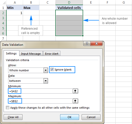
In many situations, if you select the Ignore blank box when defining the rule (usually selected by default) and one or more cells referenced in your formula is blank, any value will be allowed in the validated cell.
Here is an example in the simplest form:
Absolute and relative cell references in data validation formulas
When setting up a formula-based Excel validation rule, please keep in mind that all cell references in your formula are relative to the upper left cell in the selected range.
If you are creating a rule for more than one cell and your validation criteria are dependent on specific cells, be sure to use absolute cell references (with the $ sign like $A$1), otherwise your rule will work correctly only for the first cell. To better illustrate the point, please consider the following example.
Supposing, you want to restrict data entry in cells D2 to D5 to whole numbers between 1 (minimum value) and the result of dividing A2 by B2. So, you calculate the maximum value with this simple formula =A2/B2, like shown in the screenshot below:
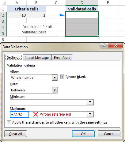
The problem is this seemingly correct formula won't work for cells D3 to D5 because relative references change based on a relative position of rows and columns. Thus, for cell D3 the formula will change to =A3/B3, and for D4 it will become =A4/B4, doing data validation all wrong!
To fix the formula, just type "$" before the column and row references to lock them: =$A$2/$B$2. Or, press F4 to toggle between different reference types.
In situations when you want to validate each cell based on its own criteria, use relative cell references without $ sign to get the formula to adjust for each row or/and column:
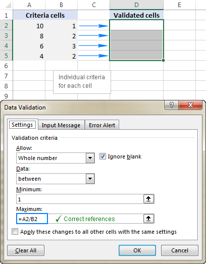
As you see, there is no "absolute truth", the same formula could be right or wrong depending on situation and your particular task.
This is how to use data validation in Excel with your own formulas. T gain more understanding, feel free to download our sample workbook below and examine the rule settings. I thank you for reading and hope to see you on our blog next week!
Practice workbook for download
Excel Data Validation examples (.xlsx file)
 by
by
203 comments
I'm trying to use data validation to not allow triplicate values in a column. Sometimes this will work and other times it doesn't and i can't figure out why!
=COUNTIF($A$1:$A$100,A1)<=2
Hello Dan!
Your formula allows two identical values in a column. To allow only one value, try the formula
=COUNTIF($A$1:$A$100,A1)<2
I have a data validation cell that references the month and year for a rolling 5 years. if I choose a month, it adds the data for each company I work with for that particular month based on an array that pulls from an Access database. I have used this workbook for 20 years. When I click on that cell to choose a new month, it used to start with the current month that was selected and then I could roll the workbook to the next month easily. Recent updates seem to have removed that feature and now it always starts at the top, so I have to scroll down several years to get to a current month. Is there a way to fix it to start on the current value that is in the cell instead of at the beginning again? Thanks!
Hello Karl!
I can't change how standard Excel tools work.If you have a specific question about a function or formula, feel free to ask, and we will do our best to assist you.
Hi Alexander, I do not think it address my curiosity.
When constructing drop down list using data validation, the “normal” approach is to create list on the same sheet or another within workbook. Like Europe, Asia, Afrika anthen only these are visible and selectable.
What I am curious about is, I have ever changing csv with options. I can use Power query to create table Anywhere in the workbook and go the “normal” way. BUT I do not like it very much, is there possibility not to create this “helper” table and use just Power query connection as source list? If yes how.
Thank you
Jindra
Hi! This can't be done with normal Excel methods. But you can experiment with VBA.
I need some help on the below case, Col A have some TAG no (repeat), Col B Material No (may or may not available in system thus valid or invalid in Col C ), I need a formula in Col D if against same TAG in Col A, Col C one of the line is In-valid then all row of the TAG in Formula (Col D) show In-Valid.
TAG Material Logic Formula
204-FOCC-101 7057581 InValid InValid
204-FOCC-101 7057581 InValid InValid
201-MCRS-201 7057583 Valid InValid
201-MCRS-201 7057583 InValid InValid
201-MCRS-101 7057583 Valid Valid
201-MCRS-101 7057583 Valid Valid
Hi! Use the IF function to get the value of a condition. To check 3 conditions for 3 columns, use the SUMPRODUCT function.
On the basis of the information given above, the formula could be as follows:
=IF(SUMPRODUCT(($A$1:$A$6=A1) * ($B$1:$B$6=B1) * ($C$1:$C$6="InValid"))>0, "InValid", "Valid")
Hi Alexander, Thanks for quick reply, I apply the formula suggested by you but not meet my requirement.
I need if any of the row against same TAG ID(Col A) Logic value is In-Valid, all the row should show as In-Valid in formula.
TAG ID COMPONENT Logic Formula
204-FOCC-101 7057581 In-Valid In-Valid
204-FOCC-101 7057581 In-Valid In-Valid
201-MCRS-201 7058233 Valid Valid
201-MCRS-201 7057583 Valid Valid
201-MCRS-101 7061604 Valid Valid
201-MCRS-101 7057583 In-Valid In-Valid
20EA-01 7061606 Valid Valid
20EA-01 7061609 In-Valid In-Valid
20EA-01 7058236 In-Valid In-Valid
20EA-01 7061607 Valid Valid
20EA-01 7062075 Valid Valid
20EA-01 7061608 Valid Valid
20EA-01 7061605 Valid Valid
Hi! You are using different data, but the proposed formula returns exactly the same data that you specified in column D. Clarify which results do not meet your requirements.
Hi All,
I would like to add a drop-down list along with allowing user to type in the cell. I was able to achieve this, however additionally I want to keep a constraint that user can only type decimal values in the cell and not alpha numeric. I can I add both this constraints in the same cell
1) Either user can select from drop-down values
2) Or he can type only decimal values in it.
Any quick help would be appreciated.
Hi! You cannot use two data validation in the same cell. You can use a drop-down list and you can use VBA code for the second validation.
I want to use the data validation tool to display the full name (e.g.,COM (Commissioning)) in the dropdown but displays the acronym in worksheet (e.g. COM). Would the custom function in data validation allow me to achieve this using 2 reference lists i.e. in full and acronym)?
Hello Lara!
To use two columns in a drop-down list and insert values from the second column, you can use a Combo Box (ActiveX Control).
On Developer tab, in Controls group, click Insert, and select Combo Box under ActiveX Controls.
Hello,
I am trying to come up with a formula to only allow a 9 digit number, or a 9 digit number with an R or G at the end. We have certin profile numbers we use at my place of work and want to make sure no one mistypes anything. For example, the entries could be 123451234 or 123121234G or 123121234R with no spaces, dashes, etc.
Hello!
We have a special tutorial that can help to solve your problem. You can find the examples and detailed instructions here: Excel Data Validation using regular expressions.
Try using this formula to data validation:
=OR(RegExpMatch(A1,"^\d{9}[RG]"), RegExpMatch(A1,"^\d{9}"))
I hope that the advice I have given you will help you solve your problem.
Hi,
Is it possible to have data validation based on the value in another cell? For example if the cell in column "Units" is "$" then allow decimal places but if not only allow whole numbers.
Thanks!
Hi! Use the IF formula for data validation. This will return TRUE or FALSE. If the remainder of the division by 1 is 0, it is an integer. You can check this with the MOD function.
Based on your information, the formula might look something like this:
=IF(A2<>"$",TRUE,MOD(B2,1)=0)
Hi
Hoping you can help, new to data validation and want to make it so when people use a drop down list of subsistence expenses they can only enter up to a certain limit. This formula worked fine: =AND(A4="Breakfast",B4<=8)=AND(A4="Lunch",B4<=10)=AND(A4="Dinner",B4<=20)
But this was in a trial spreadsheet not the main form. I transferred it to the main form (altering the cell references) and it just wouldn't work - if you enter anything at all in the validated cell it returns the error message. Thought I might have the issue in that there was another option "Other" in the drop down menu not covered in the formula. Went back to my test sheet and added it:
=AND(A4="Breakfast",B4<=8)=AND(A4="Lunch",B4<=10)=AND(A4="Dinner",B4<=20)=AND(A4="Other",B4<=10000) this ruined the data validation in my test spreadsheet too. When I paste it into a cell to test it - it works ok - what am I doing wrong?
Hi! Your AND formula is written incorrectly. Please take a look at this guide: Using the AND function in Excel. You can also find useful information in this article: Multiple AND & OR statements in one formula. For example:
=OR(AND(A4="Breakfast",B4<=8),AND(A4="Lunch",B4<=10),AND(A4="Dinner",B4<=20))
Thank you for your help ?
Hello Alexander,
Hope you are doing good.
Is it possible to change the dropdown list of your data validation depending on another cell? e.g.: For cell C15 I need to select one of the options from the list A1:A3. If I select A1 in cell C2, then the dropdown list B1:B3 will show in cell C3. But if I select A2 in cell C2, then the dropdown list C1:C3 will show in C3.
Thank you in advance for your support.
Hi! We have some instructions to help you solve your problem: How to make a dependent (cascading) drop-down list in Excel or Create a dynamic dependent drop down list in Excel an easy way.
Hello. Imagine we have a short list of strings in ColA (eg A2:A10). And this is the validation list for multiple columns, say B2:B100, C2:C100 and D2:D100. I'd like to have the dropdown for the cells in the same row in B, C and D (say B2, C2 and D2) such that when a value from the A2:A10 list is selected in B2, then the dropdown in C2 and D2 show all A2:A10 values except the one set in B2. Likewise for the value set in C2, should be missing along with B2 value from D2 possible dropdown values. In each row, the dropdowns should be such that it is not possible to have identical values from the A2:A10 list.
Thanks a lot!
Hello! To enter only unique values in multiple drop-down lists in cells B2,C2,D2, create an additional list by using the formula:
=UNIQUE(VSTACK(A2:A10,TRANSPOSE(B2:D2)),FALSE,TRUE)
If this formula will be written in K2, for example, use this reference for the drop-down list: =$K$2#
With the TRANSPOSE function you get a vertical list of values. With the VSTACK function, you combine two lists into one. The UNIQUE function creates a list of unique values for your drop-down list.
For more information, please visit: How to make a dynamic dependent dropdown list in Excel an easy way.
Thank you very much for your reply Alexander. I was initially able to make it work for a single row with a combination of COUNTIF and UNIQUE on a helper column using similarly a spill array as validation reference. Unfortunately my code does not work for the subsequent rows (B3-D3, B4-D4, etc). I notice your solution is very elegant, but seems to have the same limitation. Is there an easy way to propagate to the rows below? Thank you again! Really appreciate your time ans expertise!
Hello! To copy a drop-down list, you can use these instructions: How to edit, copy and delete drop down list in Excel. To use the same data for all dropdowns, use absolute references in the formula. Read more here: How to copy formula in Excel with or without changing references. For example, $A$2:$A$10 instead of A2:A10.
Thank you Alexander, I have solved adapting your formula this way:
=TRANSPOSE(UNIQUE(VSTACK($A$2:$A$10,TRANSPOSE($B2:$D2)),FALSE,TRUE))
this will make the spill array to develop horizontally along row 2 (for example). Then I drag down in the sheet along column F, so each row, starting in col F has a fresh spill array of my validation data in A2:A10.
I then set the validation data source for the first set of cells B2:D2 as:
=F$2#
I then select these three cells and drag down. Now any row will validate against an independent spill array on the neighboring column F without interference of the selected data of a row with those of another (for example B7:D7, will validate against F7, B11:D11 against F11 etc.)
Thank you very much for your inupts!
....Correction:
"I then set the validation data source for the first set of cells B2:D2 as:
=$F2# "
Hi!!!
How to create in excel sheet, if one cell is selected, the other column in question will function as per its formula, if not the column should not function as per formula.
Example: IF D3 is written as LSMGO, then the column G should function as per the formulas in all the cells of the column G, If the D3 is written as VLSFO, then column G should NOT function as per the formulas and cells in Column should indicate 0.
Hi! You must add an IF function with the condition you describe to each formula in column G. Data validation cannot affect the result returned by the formula.
Have dropdown list in Cell A1 and Cell C1. When i select lets say Male in cell A1, cell C1 will show a dropdown list with the list of Male. But if i change the value in cell A1 to Female, Cell C1 should be empty. however when i click on the dropdown list in cell C1 it will display the list of Femae.
Hi! If I understand your task correctly, the following tutorial should help: How to make a dependent (cascading) drop-down list in Excel.
I can't quite believe Excel doesn't have a more robust, localized Phone Number validation solution. All the existing solutions EITHER:
a) force the user to ONLY enter numerics (so they can't enter interstitial hyphens or parens) but accurately prevent leading zeros (by setting validation rule to have min & max hole number values), or
b) prevent a user from entering anything other than a numeric (by using the phone number format plus the =AND(ISNUMBER(B2),LEN(B2)=10) data validation formula), but which allows leading zeros.
c) allow illegal alphas to limit the data validation purely according to text string length.
Why can't there be a phone-specific, built in validation that:
limits input patterns to 1234567890, 123-456-7890, (123) 456-7890, (123)456-7890 but does not allow any leading zero entries nor any other alpha characters that are illegal in US phone numbers. Maybe there are other US patterns I'm not thinking about (I'm ignoring the hipster 123.456.7890 notation). The country-specific localization rules would have to allow for alternative patterns and either allow or disallow leading zeros as appropriate.
You bet there is a way...
=AND(ISNUMBER(SUBSTITUTE(SUBSTITUTE(SUBSTITUTE(A1,"(",""),")",""),"-","")+0), LEN(SUBSTITUTE(SUBSTITUTE(SUBSTITUTE(A1,"(",""),")",""),"-",""))=10)
Hi,
I have various tables in my workbook, one table is Called "All Concrete". All Concrete has sub divisions below it. When you select "All Concrete" in C3 from a drop down list my data validation formula in D3 is as follows with list selected =Indirect(substitute(C3," ","")). Excel reverts with "there's a problem with this formula". The problem is in other workbooks this works perfectly. I made a new workbook and tested the formula and it worked. When I copy all the other data in the workbook suddenly it goes back to the problem with the formula. I am very far from expert user and would appreciate a possible answer in layman's terms. Thanks
Apologies, the current workbook uses these formulas in other cells with no problem.
Hello Mr. Alexander, and I hope you have a great day ahead of you. I actually need your dire help regarding the data validation formula.
Here is my problem, now that I have a formula that only allows 1 number not greater or lesser than 1 (negative numbers) but, however, I have tried to add another "1" on older cell, for example, I have added 1 on C17 and when I want to add 1 before C17 which is C16 it shows an error message, which is that what I want to implement when I add greater than 1 or some negative numbers.
Here is my current formula: "=AND(SUM(C5:C17)=1)" and I want to solve this particular issue for my monitoring.
Hi! I don't really understand your problem. Your formula allows only one number 1 to be written into the range C5:C17 and only in one cell. What do you want to do?
Hello sir, sorry for the unclear statement.
Actually, I have this monitoring Excel file for a specific department as requested by the department's manager. And this monitoring can be used to overseer the stocks of those inks. What we ask this department staff is to request only 1 ink after their current ink is empty so we can properly handle the ink stocks and proceed to encode the date released. They cannot request more than one ink.
So the kind of Data Validation I implement is if the value exceeds to greater than 1, an error message will appear stating, "invalid request". Again, sorry for not explaining clearly earlier.
I add 1 on C17 there's no error message but, when I add 1 on C16 and other cells before it, it gave me an error message.
Am I doing it wrong or can I have a proper formula about it?
Hi,
I have created a formula that returns true and false when desired. However, when applied in the data validation, it only partially works.
I have a cell E4 in which the person inputs a list. The list format is string, string, string. For instance, E4 = Group 2, Team B, XZZ
Then, in E5, the person must type strings that belong in the listed strings in E4. Same list format. For instance, E5 = XZZ, Group 2
I want to ensure that indeed the strings used in E5 are strings that exist in E4, and case sensitive.
To do so, I came up with the following formula:
=EXACT(TEXTJOIN(", ";TRUE;IFNA(VLOOKUP(TEXTSPLIT($E5;;", ");TEXTSPLIT($E$4;;", ");1;FALSE);"#pb#"));$E5)
The formula returns TRUE, because indeed E5 (XZZ, Group 2) is made of strings that belong in E4 ( Group 2, Team B, XZZ) and respect the list format (string, string, string).
However, when I use this formula for data validation, it returns an error. The input in E5 is invalid according to the data validation.
If I have only 1 string in E5, for instance E5= XZZ, then the data validation does NOT return an error.
I don't understand why the formula works in the sheet but not in data validation.
Thanks for your help.
Hi! If E5= XZZ, then your formula returns TRUE. Therefore, the data validation does not return an error. This is consistent with the conditions you described. "XZZ" is present in "Group 2, Team B, XZZ".
Hi, I want to create a validation where each cell cannot be greater than a certain number (say 10) and the sum of certain numbers in the same range also cannot be greater than a certain number. For Eg: User has to input a number from A5 to A10, where each cell value cannot be greater than 10 and the sum of cells A5 to A10 also cannot be greater than 10. Is there a way to do this?
Hello! Create a data validation rule in cell A5 using a formula:
=AND(SUM(A5:A10)<=10,A5<=10)
Create similar rules in cells A6:A10.
Hi
I created a drop down (Data validation - list) which is link with a list of companies.
However, the dropdown menu is not in alphabetical order.
How can we have it in alphabetical order?
Thank you
Melvin
Hi! Sort the list of companies, then the dropdown list will be sorted as well. Read more: How to sort in Excel by row, column names and in custom order or Excel SORT function - auto sort data using formula.
Sir/ma'am,
I trying to create a drop down list that allows people to insert a hyperlink into a cell and then select a friendly name via drop down list within the same cell.
What I have encountered is when data validating that cell it works but when a hyperlink is inserted the data validation in that cell is over written and drop list is removed.
Hi! A drop-down list can only insert text or a number into a cell. You can use this data to create a hyperlink in another cell.