In this tutorial, you will learn how to create a dynamic named range in Excel and how to use it in formulas to have new data included in calculations automatically.
In last week's tutorial, we looked at different ways to define a static named range in Excel. A static name always refers to the same cells, meaning you would have to update the range reference manually whenever you add new or remove existing data.
If you are working with a continuously changing data set, you may want to make your named range dynamic so that it automatically expands to accommodate new entries or contracts to exclude removed data. Further on in this tutorial, you will find detailed step-by-step guidance on how to do this.
How to create a dynamic named range in Excel
For starters, let's build a dynamic named range consisting of a single column and a variable number of rows. To have it done, perform these steps:
- On the Formula tab, in the Defined Names group, click Define Name. Or, press Ctrl + F3 to open the Excel Name Manager, and click the New… button.
- Either way, the New Name dialogue box will open, where you specify the following details:
- In the Name box, type the name for your dynamic range.
- In the Scope dropdown, set the name's scope. Workbook (default) is recommended in most cases.
- In the Refers to box, enter either OFFSET COUNTA or INDEX COUNTA formula.
- Click OK. Done!
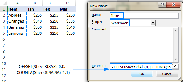
In the following screenshot, we define a dynamic range named Items that accommodates all cells with data in column A, except for the header row:

OFFSET formula to define an Excel dynamic named range
To make a dynamic named range in Excel, you can use the following generic formula:
Where:
- first_cell - the first item to be included in the named range, for example $A$1.
- range - an absolute reference to the entire column such as $A:$A if your data starts in row 1; or an absolute range reference like $A$2:$A$2000 if your data begins in some other row.
This formula leverages the COUNTA function to count the non-blank cells in the specified column, and this count is used for the height argument in OFFSET, specifying how many rows to include in the range.
For instance, to create a dynamic named range starting in cell A1 of Sheet3, use this formula:
=OFFSET(Sheet3!$A$1, 0, 0, COUNTA(Sheet3!$A:$A), 1)
If there is some data above the topmost cell of your range, adjust for it by subtracting the corresponding number of rows from COUNTA's result.
For example, if there is a single header row and the data starts in A2, subtract 1:
=OFFSET(Sheet3!$A$2, 0, 0, COUNTA(Sheet3!$A:$A) -1, 1)
For two header rows, with the data starting in A3, adjust by subtracting 2:
=OFFSET(Sheet3!$A$3, 0, 0, COUNTA(Sheet3!$A:$A) -2, 1)
Alternatively, you can provide a range to the COUNTA function that exceeds the expected maximum number of values in the dynamic range. For example:
=OFFSET(Sheet3!$A$2, 0, 0, COUNTA(Sheet3!$A$2:$A$2000), 1)
If you're defining the range for the use withing the current worksheet (Scope is set to a particular sheet), you can omit the sheet name, as Excel will handle it automatically. If the Scope is set to Workbook, be sure to include the sheet name followed by an exclamation point before the cell reference (as shown above).
Usage notes:
For the formula to work correctly, make sure that:
- There are no blank cells between data entries in the referenced column.
- There is no other data below the cells intended for your dynamic range.
INDEX formula to make a dynamic named range in Excel
Another way to create an Excel dynamic range is using COUNTA in combination with the INDEX function.
This formula consists of two parts:
- On the left side of the range operator (:), place the hard-coded starting reference like $A$2.
- On the right side, you use the INDEX function to figure out the ending reference. Here, you supply the entire column A for the array and use COUNTA to get the row number (i.e. the number of non-empty cells in column A).
For our sample dataset, the formula goes as follows:
=$A$2:INDEX($A:$A, COUNTA($A:$A))
Since there are 5 non-blank cells in column A, including a column header, COUNTA returns 5. Consequently, INDEX returns $A$5, which is the last used cell in column A (usually an Index formula returns a value, but the reference operator forces it to return a reference). And because we have set $A$2 as the starting point, the final result of the formula is the range $A$2:$A$5.
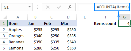
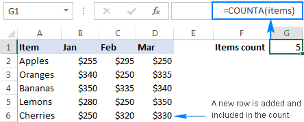
To test the newly created dynamic range, you can have COUNTA fetch the items count:
=COUNTA(Items)

If all done properly, the result of the formula will change once you add or remove items to/from the list:

Please keep in mind that for correct work of the formula, the referenced column should not contain any additional data below the dynamic range cells.
Note. While both formulas discussed above yield the same result, there is a performance difference to consider. OFFSET is a volatile function, meaning it recalculates with every change to the sheet. On modern, high-performance machines with reasonably sized datasets, this generally won't cause issues. However, on low-capacity machines or with large datasets, this recalculation may slow down Excel. In such cases, using the INDEX function to create a dynamic named range is a more efficient option.
How to make two-dimensional dynamic range in Excel
To build a two-dimensional named range, where not only the number of rows but also the number of columns is dynamic, use the following modification of the INDEX COUNTA formula:
In this formula, you have two COUNTA functions to get the last non-empty row and last non-empty column (row_num and column_num arguments of the INDEX function, respectively). In the array argument, you feed the entire worksheet (1048576 rows in Excel 365 - 2007; 65535 rows in Excel 2003 and lower).
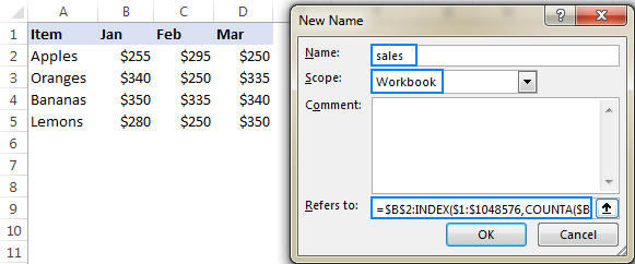
And now, let's define one more dynamic range for our data set: the range named sales that includes sales figures for 3 months (Jan to Mar) and adjusts automatically as you add new items (rows) or months (columns) to the table.
With the sales data beginning in column B, row 2, the formula takes the following shape:
=$B$2:INDEX($1:$1048576,COUNTA($B:$B),COUNTA($2:$2))

To make sure your dynamic range works as it is supposed to, enter the following formulas somewhere on the sheet:
=SUM(sales)
=SUM(B2:D5)
As you can see in the screenshot below, both formulas return the same total. The difference reveals itself in the moment you add new entries to the table: the first formula (with the dynamic named range) will update automatically, whereas the second one will have to be updated manually with each change. That makes a huge difference, uh?

How to use dynamic named ranges in Excel formulas
In the previous sections of this tutorial, you have already seen a couple of simple formulas that use dynamic ranges. Now, let's try to come up with something more meaningful that shows the real value of an Excel dynamic named range.
For this example, we are going to take the classic INDEX MATCH formula that performs Vlookup in Excel:

…and see how we can make the formula even more powerful with the use of dynamic named ranges.
As shown in the screenshot above, we are attempting to build a dashboard, where the user enters an item name in H1 and gets the total sales for that item in H2. Our sample table created for demonstration purposes contains only 4 items, but in your real-life sheets there can be hundreds and even thousands of rows. Furthermore, new items can be added on a daily basis, so using references is not an option, because you'd have to update the formula over and over again. I'm too lazy for that! :)
To force the formula to expand automatically, we are going to define 3 names: 2 dynamic ranges, and 1 static named cell:
Lookup_range: =$A$2:INDEX($A:$A, COUNTA($A:$A))
Return_range: =$E$2:INDEX($E:$E, COUNTA($E:$E))
Lookup_value: =$H$1
Note. Excel will add the name of the current sheet to all references, so before creating the names be sure to open the sheet with your source data.
Now, start typing the formula in H1. When it comes to the first argument, type a few characters of the name you want to use, and Excel will show all available matching names. Double-click the appropriate name, and it will be inserted in the formula right away:

The completed formula looks as follows:
=INDEX(Return_range, MATCH(Lookup_value, Lookup_range, 0))
And works perfectly!

As soon as you add new records to the table, they will be included in your calculations at once, without you having to make a single change to the formula! And if you ever need to port the formula to another Excel file, simply create the same names in the destination workbook, copy/paste the formula, and get it working immediately.
Tip. Apart from making formulas more durable, dynamic ranges come in handy for creating dynamic dropdown lists.
This is how you create and use dynamic named ranges in Excel. To have a closer look the formulas discussed in this tutorial, you are welcome to download our sample workbook below. I thank you for reading and hope to see you on our blog next week!
 by
by
32 comments
I have a sheet that pulls data from another sheet and place them in column A, B, C and D, starting from row 10 to row 513, where names are in column B. The rows 515 and 517 are chosen for writing signatures.
The list of names (B10:B513) in this sheet can expand or contract thus, leaving blank cells with empty string (" ").
Which formula can help me to print a range A1:F517 by excluding all blank cells but the rows 515 and 517 should appear automatically just below the last name and, what can I handle this just when I am about to print a document?
Hi! If I understand what you're asking correctly, the formula below will help you with your task:
=FILTER(A1:D517,B1:B517<>"")
You can find the examples and detailed instructions here: How to filter out blanks in Excel.
Hello.
Please I'd like to create a dynamic range from two separate ADDRESS functions for use in an INDEX & MATCH function. I'd then like to use this range in the MATCH function. I'm doing this so that I can automate the process of collating different items based on the dynamic lookup-item in MATCH function.
The ADDRESS functions are working good, so also is the MATCH and INDEX functions; but it all falls apart when I try to combine them like:
INDEX(b3: w30, MATCH(c4, (ADDRESS((d5-1),7)) : (ADDRESS((d5+10),7)), 0), 20).
Please how can I achieve creating the dynamic range for the MATCH Function?
Thank you.
Hello! To create a dynamic range reference, use the INDIRECT function. For example, for your data:
=INDIRECT(ADDRESS((D5-1),7)&":"&ADDRESS((D5+10),7))
Hello. Is it possible to store the values of a dynamic array in a named range already calculated? For example, when I enter this formula for a new named range, the name manager shows the values as an ellipsis:
=ABS(INDEX(A$1:A$1000,0,1))
I'm assuming this means Excel will recalculate that formula each time the name is referenced. Is there a way to avoid this without first having to create a column with the absolute values already calculated, and then pointing the new name to that column?
Thank you.
Hi! If I understand the question correctly, such a formula can work:
=ABS(namedrange)
or
=ABS(INDEX(namedrange,0,1))
I'm trying to add a formula in the cell following a sequence formula that is dynamic. The sequence formula can autofill in 6 cells (I want to add the formula in the 7th cell) of the sequence formula can autofill in 8 cells (I want to add the formula in the 9th cell).
Is there a way to do that automatically?
Hi! You cannot automatically add a formula to a cell.
I'm trying to do a graph to display the last 6 days worth of data using OFFSET. The formula works if I have 6 or more days in my table, but I'm receiving reference errors if I have less than 5 days.
E9=01Jan2023
F9=02Jan2023
G9=03Jan2023
H9=04Jan2023 .....
this is my formula.
=OFFSET($E$9,,IF(COUNTA($E$9:$GA$9)<6,0,COUNTA($E$9:$GA$9)-6),,IF(COUNTA($E$9:$GA$9)<6,COUNTA($E$9:$GA$9),6))
would you be able to identify where my problem lies or how I can display the graph with only 1, 2, 3, 4 or 5 days worth of data without error message?
I tested your formula with three dates in cells E9:G9 and got no error.
Hi,
I have production report with two columns one column for dates and second column is for case number so I need result how many case number completes for the date.
Example.
A column B column
03/13/23 AS123
03/13/23 AS234
03/14/23 AS768
I need countifs formula for with match date on second sheet.
Hi!
For the answer to your question and examples of formulas, see here: Using Excel COUNTIF function with dates.
Good day, I need some assistance please...I have an excel sheet with Dynamic columns. I display the total Working hours in columnD and only display the overtime hours if there are any. If there isn't any overtime hours then I display the week in days starting from either column E or columnG. I need to sort the days of the week according to a date range which I have just specified. So, If my Monday falls on the 19th and my Thursday falls on the 13th, I need to sort the columns so that Thursday comes first and Wednesday comes last. I don't know the column letter (could be D or E or F or G or so on) but I can determine the letter. I don't want to use the letter but when I substitute, I get an error. When I run the hardcoded substitution, it works fine "Sheets(sheetName).Range("I2:O132").Sort Key1:=Range("I2:O2"), Order1:=xlAscending, Orientation:=xlLeftToRight". When I use the following, I get an error Sheets(sheetName).Range(("""" & strColumnStart & "" & ":" & "" & strColumnEnd & """")).Sort Key1:=Range("""" & strColumnStart & "" & ":" & "" & strColumn & """"), Order1:=xlAscending, Orientation:=xlLeftToRight. When I use the immediate window, """" & strColumnStart & "" & ":" & "" & strColumnEnd & """" equates to "I2:O132" but it just doesn't work. Does anyone have a solution to this?
Hi!
Unfortunately, we can only help with writing Excel formulas. Your problem cannot be solved with formulas.
HI,
I have created a table using dynamic range. I would like to format(meaning color/borders) like a when I create a table with alternating fill colors for row. Is there a simple method?
The button Labeled "Format as Table" creates a table them my Dynamic range goes to Spill Error...
Thanks,
Jmarc
Hello!
You cannot create an Excel table from a named range. You need to convert formulas to values. Or use standard Excel formatting tools.
Here is the article that may be helpful to you: Highlight every other row in Excel using conditional formatting.
I'm having trouble entering the formula for a dynamic range.
=Sheet1!ADDRESS(MATCH(TODAY():$P:$P,0),16):INDEX($P:$P, COUNTA($P:$P))
or
=Sheet1!ADDRESS(MATCH(TODAY(),P10:P374,0),16):$P$374
Keeps giving me a message about am I trying to enter a formula, must start with= or -.
When I enter only the cell formula, it takes it, but I need a range.
=Sheet1!ADDRESS(MATCH(TODAY():$P:$P,0),16) Works to give the cell address of today's date.
This creates dynamic range starting at today's date in column P and I want to extend it to the end of the data in column P. Column P is a list of dates.
I need this to then find the next value in a different column after the today's date row.
This different than most dynamic ranges that only extend the bottom. I want to do both. One to move the top based on today's date and the bottom to extend it based on data being added.
I hope you can help me. I've learned a lot from you.
Thanks,
Colt
Hello!
If your list of dates starts in cell A1, then you can use the formula to create a dynamic range starting from the current date:
=OFFSET(A1,MATCH(TODAY(),A1:A300,0)-1,0, COUNTA(A1:A300)-MATCH(TODAY(),A1:A300,0)+1,1)
This should solve your task.
Hi,
How can I get the Defined Name to work for a dynamic range when I have both Blank and Non-Blank cells within my range?
Hello!
Try using the COUNTBLANK function in your dynamic range formula:
OFFSET(first_cell, 0, 0, COUNTA(column)+COUNTBLANK(column), 1)
I hope it’ll be helpful.
I don't think this will work. The COUNTBLANK function will also count all of the blanks below the last item in the column giving you a very large value for modern versions of Excel.
Hi!
Of course, you can use a range of cells instead of the entire column in the formula.
For example - Instead of COUNTA(column) use COUNTA(A1:A100)
This will seriously speed up the calculations.
I would like to add numbers in a column
using sum, offset, counta and the column has a name.
For practice, I have column E and beginning with row 3 the title: salary. Rows 4, 5, 6,etc are the salaries. Column E3:E10 has been named as "monthly_salaries". I need to use that so I can place the sum(monthly_salaries) function on any worksheet, while the monthly-salaries will be on a seperate worksheet.
Each month the length of this vertical column E changes as more or less people draw salaries. Also, I use different worksheets so data, like the salaries may be located on worksheet 2 and the actual sum on worksheet 1.
I have offset(e3,0,0,counta(E:E),1.
Question: How to combine the column name with the sum function to accommodate the dynamic nature of this problem.
Thank you for your assistance.
Chris
Hello!
Create a dynamic named range “monthly_salaries” using a formula
=OFFSET($E$3, 0, 0, COUNTA($E$3:$E$10), 1)
Use it like this:
=SUM(monthly_salaries)
I hope I answered your question.
hi there.. hope someone could help me. I want to create a name in my file which is getting values from a single column table. I want to exclude one specific value and don't want it to be part of the name range. Not sure how can I do that? Column data is:
Fruits (table header)
Apple
Banana
Orange
Grapes
Want to have a list that exclude "Orange". As it's a table I will be adding new names after Grapes in near future.
Pls refer to: FILTER(A1:INDEX(A:A,COUNTA(A:A)),A1:INDEX(A:A,COUNTA(A:A))"Orange") in the New Name dialog
I have a simple table: 7 columns, 4 rows. Can I create a formula just adding Hrs of bananas?
Jan 1 Jan 2 Jan 3
Hrs Cases Hrs Cases Hrs Cases
Bananas 1 10 3 30 0 0
Apples 5 20 1 4 3 12
_______|___Hrs_|_Cases_|_Hrs_|_Cases_|_Hrs_|_Cases
Bananas|____1__|___10__|__3__|___30___|_0__|___0__
Apples_|____5__|___20__|__1__|___04___|_3__|___12_
No sure if this will help to understand the table...
An easy way to do it if you need a range is to use indirect in the name.. eg example for A2:G10
There is 20 rows in coloumn A
=Indirect(Sheet_name!A2:G"&CountA(A:A))
since indirect "translate" the expression - so it reads the name to be refered to this
Sheet_name!A2:G10
Correction - There is 20 rows in coloumn A - should ofcourse be 10 rows ;)
I'm trying to create a dynamic range showing client names only if their status is Active in another column. Can someone help me with the formula for this?
Pls refer to: FILTER(A1:INDEX(A:A,COUNTA(A:A)),B1:INDEX(B:B,COUNTA(B:B))="Active") in the New Name dialog