The tutorial shows how to extract number from various text strings in Excel by using formulas and the Extract tool.
When it comes to extracting part of a text string of a given length, Excel provides three Substring functions (Left, Right and Mid) to quickly handle the task. When it comes to extracting numbers from an alphanumeric string, Microsoft Excel provides… nothing.
To get a number from a string in Excel, it takes a little ingenuity, a bit of patience, and a bunch of different functions nested into each other. Or, you can run the Extract tool and have the job done with a mouse click. Below you will find full details on both methods.
How to extract number from the end of text string
When you have a column of alphanumeric strings where number comes after text, you can use the following formula to get it.
We will dwell on the formula's logic a bit later. For now, simply replace cell with a reference to the cell containing the original string (A2 in our case), and enter the formula in any empty cell in the same row, say in B2:
=RIGHT(A2, LEN(A2) - MAX(IF(ISNUMBER(MID(A2, ROW(INDIRECT("1:"&LEN(A2))), 1) *1)=FALSE, ROW(INDIRECT("1:"&LEN(A2))), 0)))
This formula gets number only from the end. If a string also has numbers in the beginning or middle, they are ignored:
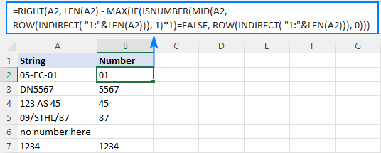
The extraction is performed with the RIGHT function that belongs to the category of Text functions. The output of this function is always text. In our case, the result is a numeric substring, which in terms of Excel is also text, not number.
If you need the result to be a number (that you can use in further calculations), then wrap the formula into the VALUE function or perform an arithmetic operation that does not change the result, say, multiply by 1 or add 0. To catch errors in the strings that do not contain a single number, use the IFERROR function. For example:
=IFERROR(VALUE(RIGHT(A2, LEN(A2) - MAX(IF(ISNUMBER(MID(A2, ROW(INDIRECT("1:"&LEN(A2))), 1)*1)=FALSE, ROW(INDIRECT("1:"&LEN(A2))), 0)))), "")
or
=IFERROR(RIGHT(A2, LEN(A2) - MAX(IF(ISNUMBER(MID(A2, ROW(INDIRECT("1:"&LEN(A2))), 1) *1)=FALSE, ROW(INDIRECT("1:"&LEN(A2))), 0))) +0, "")
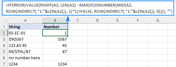
Note. In Dynamic Array Excel (Office 365 and 2021), you enter the formula in the usual way with the Enter key. In Excel 2019 and earlier, it only works as an array formula, so remember to press Ctrl + Shift + Enter to complete it.
How this formula works:
To extract number from an alphanumeric string, the first thing you need to know is where to start the extraction. The position of the last non-numeric character in a string is determined with the help of this tricky formula:
MAX(IF(ISNUMBER(MID(A2, ROW(INDIRECT("1:"&LEN(A2))), 1)*1)=FALSE, ROW(INDIRECT("1:"&LEN(A2))), 0))
To understand the logic, let's investigate it from the inside:
The ROW(INDIRECT("1:"&LEN(A2))) combination creates a sequence of numbers corresponding to the total of characters in the source string (A2), and we serve these sequential numbers to MID as the starting numbers:
MID(A2, {1;2;3;4;5;6;7;8}, 1)
The MID function pulls each individual character from A2 and returns them as an array:
{"0";"5";"-";"E";"C";"-";"0";"1"}
As MID is a text function, its output is always text (as you can notice, all the characters are enclosed in quotation marks). To turn numeric ones into numbers, we multiply the array by 1 (double negation --MID() will have the same effect). The result of this operation is an array of numbers and #VALUE! errors representing non-numeric characters:
ISNUMBER({0;5;#VALUE!;#VALUE!;#VALUE!;#VALUE!;0;1})
The ISNUMBER function evaluates each element of the array and gives its verdict in the form of Boolean values - TRUE for numbers, FALSE for anything else:
{TRUE;TRUE;FALSE;FALSE;FALSE;FALSE;TRUE;TRUE}
This array goes to the logical test of the IF function, where each element of the array is compared against FALSE:
IF({TRUE;TRUE;FALSE;FALSE;FALSE;FALSE;TRUE;TRUE}=FALSE, ROW(INDIRECT("1:"&LEN(A2))), 0)
For each FALSE (non-numeric value), another ROW(INDIRECT()) function returns its relative position in the string. For each TRUE (numeric value), a zero is returned. The resulting array looks as follows:
{0;0;3;4;5;6;0;0}
The rest is easy. The MAX function finds the highest number in the above array, which is the position of the last non-numeric value in the string (6 in our case). Simply, subtract that position from the total length of the string returned by LEN, and pass the result to RIGHT to let it know how many characters to extract from the right side of the string:
RIGHT(A2, LEN(A2) - 6)
Done!
How to extract number from the beginning of text string
If you are working with records where text appears after number, you can extract number from the start of a string by using this generic formula:
With the original string in A2, use the following formula to get number:
=LEFT(A2, MATCH(FALSE, ISNUMBER(MID(A2, ROW(INDIRECT("1:"&LEN(A2)+1)), 1) *1), 0) -1)
No matter how many digits are in the middle or end, only the starting number is extracted:

Note. In Excel 365 and Excel 2021, due to support for dynamic arrays, a regular formula works fine. In Excel 2019 and earlier, you should press Ctrl + Shift + Enter to explicitly make it an array formula.
How this formula works:
Here, we again use the combination of ROW, INDIRECT and LEN functions to create a sequence of numbers equal to the total of characters in the source string plus 1 (the role of that additional character will become clear a bit later).
ROW(INDIRECT("1:"&LEN(A2)+1))
MID and ISNUMBER do the same job as in the previous example - MID pulls individual characters and ISNUMBER converts them to the logical values. The resulting array of TRUE's and FALSE's goes to the MATCH function as a lookup array:
MATCH(FALSE, {TRUE;TRUE;FALSE;FALSE;FALSE;FALSE;TRUE;TRUE;FALSE}, 0)
MATCH computes a relative position of the first FALSE, giving us the position of the first non-numeric character in the string (3 in A2). To extract the preceding numbers, we subtract 1 from position the first text character and serve the difference to the num_chars argument of the LEFT function:
LEFT(A2, 3-1)
Now, back to an "extra" character in the sequence generated by ROW(INDIRECT()+1)). As you already know, this sequence provides the starting points for the MID function. Without +1, MID would extract exactly as many characters as there are in the original string. If the string contains only numbers, ISNUMBER will return only TRUE's while MATCH needs at least one FALSE. To ensure that, we add one more character to the total length of the string, which the MID function would convert to an empty string. For example, in B7, MID returns this array:
{"1";"2";"3";"4";""}
Note. As is the case with the RIGHT function, LEFT also returns a numeric substring, which is technically text, not number. To get the result as a number rather than a numeric string, nest the formula in the VALUE function or multiply the result by 1 as shown in the first example.
How to get number from any position in a string
If your task implies extracting number from anywhere in a string, you can make use of the following mind-boggling formula published on MrExcel forum:
=SUMPRODUCT(MID(0&A2, LARGE(INDEX(ISNUMBER(--MID(A2, ROW(INDIRECT("1:"&LEN(A2))), 1)) * ROW(INDIRECT("1:"&LEN(A2))), 0), ROW(INDIRECT("1:"&LEN(A2))))+1, 1) * 10^ROW(INDIRECT("1:"&LEN(A2)))/10)
Where A2 is the original text string.
Breaking down this formula would require a separate article, so you can simply copy it to your worksheet to make sure it really works :)
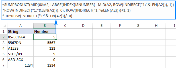
Upon examining the results, however, you may notice one insignificant drawback - if the source string does not contain a number, the formula returns zero, as in row 6 in the screenshot above. To fix this, you can wrap the formula in the IF statement, the logical test of which checks if the source string contains any number. If it does, the formula extracts the number, otherwise returns an empty string:
=IF(SUM(LEN(A2)-LEN(SUBSTITUTE(A2, {"0","1","2","3","4","5","6","7","8","9"}, "")))>0, SUMPRODUCT(MID(0&A2, LARGE(INDEX(ISNUMBER(--MID(A2,ROW(INDIRECT("$1:$"&LEN(A2))),1))* ROW(INDIRECT("$1:$"&LEN(A2))),0), ROW(INDIRECT("$1:$"&LEN(A2))))+1,1) * 10^ROW(INDIRECT("$1:$"&LEN(A2)))/10),"")
As shown in the screenshot below, the improved formula works beautifully (kudos to Alex, our Excel guru, for this improvement):
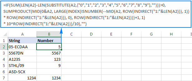
Unlike in all previous examples, the result of this formula is number. To make sure of this, just notice the right-aligned values in column B and truncated leading zeros.
Tip. In Excel 365 - Excel 2019, there is a much simpler solution with the help of the TEXTJOIN function. Please see How to remove text and keep numbers.
Extract number from text string with Ultimate Suite
As you have just seen, there is no trivial Excel formula to pull number from a text string. If you have difficulties with understanding the formulas or tweaking them for your data sets, you may like this simple way to get number from string in Excel.
With our Ultimate Suite added to your Excel ribbon, this is how you can quickly retrieve number from any alphanumeric string:
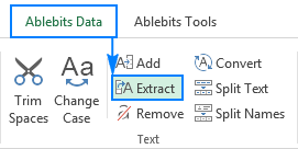
- Go to the Ablebits Data tab > Text group, and click Extract:
- Select all cells with the source strings.
- On the Extract tool's pane, select the Extract numbers radio button.
- Depending on whether you want the results to be formulas or values, select the Insert as formula box or leave it unselected (default).
My advice is to select this box if you want the extracted numbers to update automatically as soon as any changes are made to the source strings. If you want the results to be independent on the original strings (e.g. in case you plan to remove the source data at a later point), then do not select this box.
- Click the Insert Results button. Done!
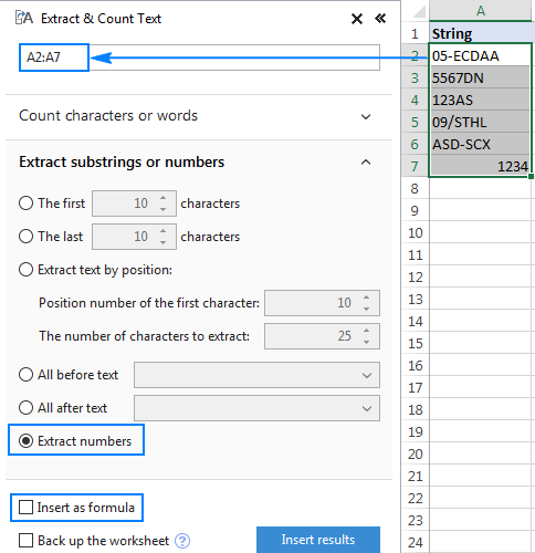
Like in the previous example, the results of the extraction are numbers, meaning you are free to count, sum, average, or perform any other calculations with them.
In this example, we've chosen to insert the results as values, and the add-in did exactly what was asked for:
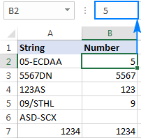
If the Insert as formula checkbox was selected, you'd observe a formula in the formula bar. Curious to know which one? Just download Ultimate Suite's trial and see for yourself :)
Available downloads
Excel Extract Number - sample workbook (.xlsx file)
Ultimate Suite - trial version (.exe file)
 by
by
577 comments
Hello,
I'm trying to extract a currency value from a text string, but having no success so far. I've used the formula above, but it extracts the entire string, and not just the numeric value.
My software is Softmaker Planmaker, which is an Excel style spreadsheet.
I also need to preserve positive from negative values, so I need the - sign where necessary.
Samples
RGE 128.72
GA-154.08
Any ideas?
AL
Hi! To extract a negative number from text in Excel, you can use a combination of Excel functions.
Use FIND function to locate the position of the negative sign (-) in the text string.
Use MID function to extract the substring starting from the negative sign.
Use VALUE function to convert the extracted text into a number.
=VALUE(MID(A1, FIND("-", A1), LEN(A1) - FIND("-", A1) + 1))
I struggling to extract number from cell, on Google sheet
condition is extracted number will not change if i change number from 1st source
Ex.
In cell A1 468.12
required B1 468.12
condition is extracted number (B1 468.12) will not change if i change number (A1 468.12) from 1st source
Hello Vishal,
Please read this article: Extract numbers from Google Sheets cells. There's also a formula-free solution for this if you're interested.
Additionally, based on the description of your task, you may find the Fill Blank Cells add-on useful.
hi - great tutorial you've put here. For my application, i want to pull from a number from a text string which has a comma in it. For example, i want the number 10,133 from the string US$10,133. Can you point me what to do? Thanks
Hello Tom!
You can extract a number with a delimiter "," from text using the formula
=TEXTJOIN("",TRUE, IFERROR(MID(A1,ROW(INDIRECT("1:"&LEN(A1))),1)*1, IF(MID(A1,ROW(INDIRECT("1:"&LEN(A1))),1)=",",",","")))
Explanation:
LEN(A1): LEN function calculates the length of the text in cell A1.
INDIRECT("1:"&LEN(A1)): INDIRECT generates an array of numbers from 1 to the length of the text in cell A1. For example, if A1 has 9 characters, it generates {1, 2, 3, 4, 5, 6, 7, 8, 9}.
ROW(INDIRECT("1:"&LEN(A1))): This creates an array of row numbers which correspond to each character in the text. So, it effectively creates {1, 2, 3, 4, 5, 6, 7, 8, 9}.
MID(A1, ROW(INDIRECT("1:"&LEN(A1))), 1): The MID function extracts each character from the text in A1 one by one. It uses the array of row numbers to do this. So, it extracts the first character, then the second, and so on.
MID(A1, ROW(INDIRECT("1:"&LEN(A1))), 1)*1: This attempts to multiply each character by 1. If the character is a number, it converts it to a numeric value. If the character is not a number (e.g., a letter or symbol), it results in an error.
IFERROR(..., IF(...)): The IFERROR function catches any errors from the multiplication step. If an error occurs (i.e., the character is not a number), the IF function checks if the character is a comma. If it is, it returns the comma; otherwise, it returns an empty string.
TEXTJOIN("", TRUE, ...): Finally, TEXTJOIN concatenates all the results together. The "" means there is no delimiter, and TRUE tells TEXTJOIN to ignore empty strings.
Hi - i solved my problem. thanks
Hi
I have a bit of a complex ask and I cant seem to get to the correct solution. I have a column which contains a set of data both letters and numbers. I am trying to extract in a new column the number from the cell ONLY if the cell contains a number that starts with 9 and contains 10 digits. If not returns a blank.
For example:
CPR OBZA/91256058 should return a blank since the number is less than 10 characters.
0912502789 should return a blank although its 10 digits it does not start with 9.
Hello Christopher!
To count the number of digits and get the first digit, extract the number from the text string using this guide: How to extract number from string in Excel.
For example, use this formula:
=TEXTJOIN("",TRUE,IFERROR(--MID(A1,ROW(INDIRECT("1:"&LEN(A1))),1),""))
Use the IF AND formula to check both conditions:
=IF(AND(LEN(TEXTJOIN("",TRUE,IFERROR(--MID(A1,ROW(INDIRECT("1:"&LEN(A1))),1),"")))=10, LEFT(TEXTJOIN("",TRUE,IFERROR(--MID(A1,ROW(INDIRECT("1:"&LEN(A1))),1),"")),1)="9"), TEXTJOIN("",TRUE,IFERROR(--MID(A1,ROW(INDIRECT("1:"&LEN(A1))),1),""))," ")
Simplified version of the formula: =TEXTJOIN("",TRUE,IF(ISNUMBER(MID(A2,SEQUENCE(LEN(A2)),1)*1)=TRUE,MID(A2,SEQUENCE(LEN(A2)),1),""))
Hi Narsimha,
Thank you for your feedback! This article was written many years ago when the TEXTJOIN function did not exist yet. I believe it can still be helpful for users of Excel 2016 and older versions. The TEXTJOIN formulas are covered in separate article: How to remove text and leave numbers or vice versa.
I have a regular need to extract costs from a shopping receipt. eg
1 Sainsbury's Pure Orange Juice 1L £1.75
1 Sainsbury's Reduced Sugar & Salt Baked Beans In Tomato Sauce £2.30
1 Sainsbury's Royal Gala Apples, SO Organic x6 £2.30
1 Sainsbury's Spicy Bean Burgers x4 454g £1.69
2 Heinz Lentil Soup 400g £3.40
2 Sainsbury's Fairtrade Bananas, SO Organic x6 £3.60
I have found by accident that Excel will let me do this very simply. I type the first number 1.75 in a cell next to the text and move to the next cell below and type 2 then at this point Excel will insert all the subsquent values in the remainder of the receipt. There are a few hiccups I have come across but they are minor compare with the ease of extracting most of the values.
Hope this helps a few of you.
Hello,
Beautiful stuff all these different formula's that I use as well. but now I have run inn to a little(...?) more complex challenge.
I need to extract the number from a serie of string separated by a blanc.
So the string in 1 cell looks like "sprint12 sprint13 sprint14 sprint15 sprint16 sprint17 sprint18 sprint19 sprint20" and I need to retrieve the separate number from each individual string.
I should therefore end with 12 13 14 15. Even more I also need to be able to select a range of predefined numbers from each individual string. For example all numbers between 14 and 17.
For 1 string I (can) use:
=SUMPRODUCT(MID(0&A2, LARGE(INDEX(ISNUMBER(--MID(A2, ROW(INDIRECT("1:"&LEN(A2))), 1))
*ROW(INDIRECT("1:"&LEN(A2))), 0), ROW(INDIRECT("1:"&LEN(A2))))+1, 1)
* 10^ROW(INDIRECT("1:"&LEN(A2)))/10)|
But as explained I need to do this in a composed string.
Very curious if someone out there can help me with my challenge.
Many thanks in advance!
Ingmar
Hi Ingmar,
You can try the below formula
=TEXTJOIN("",TRUE,IF((ISNUMBER(MID(A2,SEQUENCE(LEN(A2)),1)*1)=TRUE)*1+(MID(A2,SEQUENCE(LEN(A2)),1)=" ")=1,MID(A2,SEQUENCE(LEN(A2)),1),""))
Hello Ingmar!
For your data, if you want to extract two-digit numbers from the text, you can split it using TEXTSPLIT function. Then extract the last 2 characters from each text string using RIGHT function and convert them to a number using a math operation.
=--RIGHT(TEXTSPLIT(A1,," "),2)
To see if the number you want is in the text, you can also use the SEARCH function. For more information, please read: How to find substring in Excel. You can create a sequence of the desired numbers from 14 to 17 using the SEQUENCE function.
=ISNUMBER(SEARCH(SEQUENCE(4,1,14,1),A1))*SEQUENCE(4,1,14,1)
Thank you so much your lesson. but i find much way that cannot solve my case. No one how to do it!
my case that is on the row have such text string by data entry
"987667 x 2, 764568 x 3, 765456, 765456 x 4, 876567 x 2, 765678"
total 6 group number(sometimes only a group, depend on the data entry)
,some have need multiple 2 or 3 or 4.
As above case the result is "13" because 1st group = 2, 2nd group = 3, 3rd group = 1, 4th group = 4, 5th group = 2, 6th group = 1
i don't know how to set the auto count because that involve many criteria inside.
Please help!
Hi! You can extract numbers that are between two characters with the help of regular expressions. You can use this guide: How to extract substrings in Excel using regular expressions (Regex). You can sum these numbers using the SUMPRODUCT function.
The formula might look as follows:
=SUMPRODUCT(--SUBSTITUTE(SUBSTITUTE(RegExpExtract(A1,"\x(.*?)\,"),",",""),"x",""))
However, you cannot extract the number 1, which is not in this text.
Thank you so much. i try to work this.
Hello,
how can i extract number if i have cells where number is at the end, somewhere is in the middle and somewhere is between other numbers.
Examples:
Torta 3.5 120 ks box 20
CHorap KS BOT 20 SLI
Tasha (3.5) KS BOX 120gr
so i need, from the first i need 20, from the second i need 20, from the third i need 120.
Best
Hello Ema!
Your data does not have a common pattern. Therefore, you must use a specific formula for each of them:
=TRIM(RIGHT(SUBSTITUTE(A2, " ", REPT(" ", LEN(A2))), LEN(A2)))
=SUMPRODUCT(MID(0&A3, LARGE(INDEX(ISNUMBER(--MID(A3, ROW(INDIRECT("1:"&LEN(A3))), 1)) * ROW(INDIRECT("1:"&LEN(A3))), 0), ROW(INDIRECT("1:"&LEN(A3))))+1, 1) * 10^ROW(INDIRECT("1:"&LEN(A3)))/10)
=LEFT(TRIM(RIGHT(SUBSTITUTE(A4, " ", REPT(" ", LEN(A4))), LEN(A4))), MATCH(FALSE,ISNUMBER(--MID(TRIM(RIGHT(SUBSTITUTE(A4, " ", REPT(" ", LEN(A4))), LEN(A4))),ROW($1:$50),1)),0)-1)
Hello, thank you for sharing all these advance formulas, which very helpful. We try to extract numeric characters from multiple positions in text strings in a large files with this formula =IF($AA4<0,SUBSTITUTE(TRIM(CONCAT(IF(ISNUMBER(--MID($F4,ROW($4:$140),1)),MID($F4,ROW($4:$140),1)," ")))," ",", "),"")
But, one trouble we have is on how not to extract the digits from date in the text strings in certain rows?
Samples: (line#4) Sale of item#12, #506, #4321 to company A 6/21/2019.
(line#92)Sale of item#13, 54, 2301 to company B on 06/05/21
the formula above resulted: 12, 506, 4321, 6, 21, 2019 and 13, 54, 2301, 6, 05, 21 respectively
But the desired result on each line item would be 12, 506, 4321 and 13, 54, 2301 respectively.
Thank you for your help in advance.
Hi! You can split the text string into individual numbers using the TEXTSPLIT function. Then use the CHOOSECOLS function to select the first 3 numbers from this array.
Based on the information given, the formula could be as follows:
=CHOOSECOLS(TEXTSPLIT(IF($AA4<0, SUBSTITUTE(TRIM(CONCAT(IF(ISNUMBER(--MID($F4,ROW($4:$140),1)), MID($F4,ROW($4:$140),1)," ")))," ",", "),""),","),1,2,3)
Thank you for the quick response and solution! However, unfortunately, using the Choosecols and Testsplit formula above couldn't address the issue completely, given that the end result the three sets of digits were spilled over into three fields/columns instead of within the same cell.
Sorry, our apologies for that we forgot to mention that the descriptions/text strings in column were one various from another: some text strings don't have a date in it at all (to which the formula we originally use above could result the desired output. Other text strings with a date embedded have various sets of numeric Characters: some had only 1 set while other haver 2 or 3 or more sets in different positions within one text string. Any suggestions on how to exclude the date when extracting various sets of numbers from the same column?
Hi! I've already answered you. Try using regular expressions.
Sorry, when used a different PC to look it up, we didn't see our reply or your 2nd reply for somehow, that was why we posted it once more... Well, we got it solved. Thanks again for your help.
Thank you for the quick response and formula! Sorry, as we forgot to mention that the descriptions in column F were not standardized because some text strings in column F don't have a date at all (to which our original formula would work), while those text strings with a date have various sets of numeric characters: some have 1 or 2, or 3, or more than 3 sets.
So, unfortunately, using the "CHOOSECOLS function to select the first 3 numbers from this array" wouldn't address the issue for the whole file. Also, for somehow, the Choosecols-textsplit formula above would cause the extracted three sets of digits to spill over into three columns (i.e. AB, AC, AD) instead of one. Any other solution?
Hi! You can combine three sets of digits into one text string using CONCAT or TEXTJOIN function.
However, it makes no sense to talk about a formula that extracts the right number of numbers from each cell if your data doesn't have a common pattern.
I can't guess what your data looks, but you can try to use a regular expressions and this instruction to extract numbers from text: Regex to extract strings in Excel (one or all matches). The formula might look as follows:
=SUBSTITUTE(TEXTJOIN(", ",TRUE, RegExpExtract(F4, "#\d+")),"#","")
I recommend paying attention to the Regex tool. You can find, extract, compare, delete, or replace strings that match the regular expression pattern you enter. You don't need to install any VBA code.
The tool is included in the Ultimate Suite for Excel and can be used in a free trial to see how it works.
Hello, I want to extract "Credit transactions - total debit: ₪11020.65"
Desired Output: 11020.65
Hello! If you want to extract not only numbers but also a specific delimiter from a text string, specify that delimiter in the formula below:
=TEXTJOIN("",TRUE, IFERROR(MID(A1,ROW(INDIRECT("1:"&LEN(A1))),1)*1, IF(MID(A1,ROW(INDIRECT("1:"&LEN(A1))),1)=".",".","")))
Hi, I want to get the sum of the numbers in a string. For example "Entertainment $500, Moderator $500, Food $188, Tech $50". I want the sum of those numbers.
Hi! To extract all numbers from a text string, you can use regular expressions. You can find the examples and detailed instructions here: How to extract substrings in Excel using regular expressions (Regex).
=SUM(--RegExpExtract(A1,"\d+"))
The numbers are extracted from the text string as text. Therefore, it is necessary to convert them to normal numbers. The formula uses this instruction: Turn text into number with mathematic operations.
I recommend paying attention to the Regex tool. You can find, extract, compare, delete, or replace strings that match the regular expression pattern you enter. You don't need to install any VBA code. The tool is included in the Ultimate Suite for Excel and can be used in a free trial to see how it works.
Doesn't seem to be working for excel 2016.
All of the things I've recommended to you will work in Excel 2016.
All the information is in 1 cell.
I also use Excel 2016.
Hey, in column C I have a text that contains number (EX: under Cell C2 "so: 1289375 kdjrg cjnds 1234 jnfe") I need to extract only the long number (1289375) to a new cell (EX:N2) in the same row. can anyone assist? I couldn't find anything helpful anywhere
Hi! Find the position of the first digit in the text using the formula:
MATCH(TRUE,ISNUMBER(--MID(A2,ROW(INDIRECT("1:"&LEN(A2))),1)),0)
Delete all characters before the first digit in the text:
MID(A2,MATCH(TRUE,ISNUMBER(--MID(A2,ROW(INDIRECT("1:"&LEN(A2))),1)),0),50)
Extract the number on the left from this text string as described in this section above: How to extract number from the beginning of text string.
=LEFT(MID(A2,MATCH(TRUE,ISNUMBER(--MID(A2,ROW(INDIRECT("1:"&LEN(A2))),1)),0),50), MATCH(FALSE, ISNUMBER(MID(MID(A2,MATCH(TRUE,ISNUMBER(--MID(A2,ROW(INDIRECT("1:"&LEN(A2))),1)),0),50), ROW(INDIRECT("1:"&LEN(MID(A2,MATCH(TRUE,ISNUMBER(--MID(A2,ROW(INDIRECT("1:"&LEN(A2))),1)),0),50))+1)), 1) *1), 0) -1)
I hope it’ll be helpful.
Hi! These formulas helped a lot and the explanation is super - I'm learning a lot from this site with the examples.
One question about how to get the number from any position in string formula.
I have this text that comes from a MS form and will be consistent values, but change based on input. So the full input would look like this:
Site X (1p);Site XX (1p);Site XXY (10p);Site XYY (8p);Site YYY (5p);
Of course, if the user inputs only "Site X", the formula correctly reads it as 1. But if I add the full text and use the formula provided above:
=SUMPRODUCT(MID(0&Form1!I2; LARGE(INDEX(ISNUMBER(--MID(Form1!I2; ROW(INDIRECT("1:"&LEN(Form1!I2))); 1)) * ROW(INDIRECT("1:"&LEN(Form1!I2))); 0); ROW(INDIRECT("1:"&LEN(Form1!I2))))+1; 1) * 10^ROW(INDIRECT("1:"&LEN(Form1!I2)))/10)
It will return 111085 in the cell as the result.
How can I add the different values to make it 25 (1+1+10+8+5) for example?
Hi! To extract all the numbers from the text and sum them, use this formula:
=SUM(--TEXTSPLIT(TRIM(CONCAT(IF(ISNUMBER(--MID(A1,ROW($1:$100),1)),MID(A1,ROW($1:$100),1)," ")))," "))
If the TEXTSPLIT function is not available in your version of Excel, you can use regular expressions as described in this guide: How to extract substrings in Excel using regular expressions (Regex).
=SUM(--RegExpExtract(A1,"\d+"))
I recommend paying attention to the Regex tool. You can find, extract, compare, delete, or replace strings that match the regular expression pattern you enter. You don't need to install any VBA code.
The tool is included in the Ultimate Suite for Excel and can be used in a free trial to see how it works.
Hi Alex!
I would like to install, but additional tools/addons are unfortunately blocked by our admin, so need to find formulas instead :)
Thank you so much for the formula! I have tested and it is working very well!!
is there a way to extract numbers before and after a specific symbol. example
Cell A1 contains
I would like to have cell B1 = .5926 and cell C1 = .5906
Thank you
Unfortunately, this information is not enough to recommend a formula to you. Please provide me with an example of the source data and the expected result.
Imported data comes into excel as:
CELL A1 = (less than symbol).5926(exclamation symbol).5906(greater than symbol)
from that imported data I require my cell B1 to be my first number in cell A1 and cell C1 to be my 2nd number in A1.
CELL B1 = .5926
CELL C1 = .5906
Currently I just copy and past the data from CELL A1 and past into CELL's B1 and C1 and delete the un-needed 3 symbols and numbers, but it can be time consuming when I have 50 or more to go through.
As I told you, to extract text between two characters, you can use the TEXTBEFORE and TEXTAFTER functions. For example:
=TEXTAFTER(TEXTBEFORE(A1,"!"),"<")
You can also use this instruction: How to extract text between two characters or words in Excel. The formula might look like this:
=MID(A1, SEARCH("<", A1)+1, SEARCH("!", A1) - SEARCH("<", A1) -1)
THANK YOU!
I had entered the TextBefore/TextAfter incorrectly in my formula. Your example has just saved me.
Have a great day!!!
Cell A1 = ""
Remove the "" from this, it did not show up in my first post
Hi! To extract numbers before and after a specific symbol, you can use the TEXTBEFORE and TEXTAFTER functions. There is not enough information for a more accurate answer.
A1 = (less than symbol).5926(exclamation symbol).5906(greater than symbol)
Sorry, it's showing blank when place my post.
Hi, how do I extract the percentage of '%cotton' within a text:
61% Recycled Polyester, 26% Lenzing Ecovero Viscose, 7% Cotton, 6% Elastane
90% cotton
70% pima cotton, 30% cotton
Thank you
Hi! Get the text in before the "% Cotton" using the SEARCH and LEFT function as described here: Get text before a specific character.
Then extract the last number from this text string as recommended in this guide: How to extract last word in Excel.
Based on your information, the formula might look something like this:
=TRIM(RIGHT(SUBSTITUTE(LEFT(A1,SEARCH("% Cotton",A1)-1), " ", REPT(" ", LEN(LEFT(A1,SEARCH("% Cotton",A1)-1)))), LEN(LEFT(A1,SEARCH("% Cotton",A1)-1))))
Hello;
I can't thank enough. This helped me a lot.
I have one question. I need to extract a text containing both letters and number, for example; RNY1K5L2KL8.
The text always starts with RNY and it's always 11 characters and always alphanumerical.
I have a data where this text needs to be extract but I can't manage to extract it. This 11 character text can be ata the begining of the cell, or at the end or in the middle somewhere in the cell. I have tried everyting except the VBA which I not really familiar, but could't extract it.
Is there anyway that I can extract it with an Excel Formula.
I would really appreciate if you can help me.
Hi! If I understand correctly, find the position number of the text string "RNY" in the cell using the SEARCH function. Then, starting from that position, extract 11 characters from the text using the MID function. Please try the following formula:
=MID(A1,SEARCH("RNY",A1),11)
Dear Alaxender;
Thank you so much! You've no idea how happy I am. May the God bless you.
I can't beleieve how simple the formula looks. I have been searching the the solution in the wrong formulas and the places.
Thank you again; have a lovely day.
Ashish7162627kumar61717yadav - 716262761717
Ankit8271sharma8546 - 82718546
mujhe only number value extract karke laani hai
how to find this number 06.436.01.0.00 in excel without doubts. means 0643601000
How would I extract "16.5697" from the following string "Hourly Pay (16.5697 hours @ $0.00/hr):"