The tutorial shows how to group rows in Excel to make complicated spreadsheets easier to read. See how you can quickly hide rows within a certain group or collapse the entire outline to a particular level.
Worksheets with a lot of complex and detailed information are difficult to read and analyze. Luckily, Microsoft Excel provides an easy way to organize data in groups allowing you to collapse and expand rows with similar content to create more compact and understandable views.
Grouping rows in Excel
Grouping in Excel works best for structured worksheets that have column headings, no blank rows or columns, and a summary row (subtotal) for each subset of rows. With the data properly organized, use one of the following ways to group it.
How to group rows automatically (create an outline)
If your dataset contains just one level of information, the fastest way would be to let Excel group rows for you automatically. Here's how:
- Select any cell in one of the rows you want to group.
- Go to the Data tab > Outline group, click the arrow under Group, and select Auto Outline.
That's all there is to it!
Here is an example of what kind of rows Excel can group:
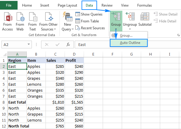
As shown in the screenshot below, the rows have been grouped perfectly and the outline bars representing different levels of data organization have been added to the left of column A.

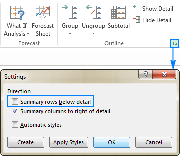
Note. If your summary rows are located above a group of detail rows, before creating an outline, go to the Data tab > Outline group, click the Outline dialog box launcher, and clear the Summary rows below detail checkbox.
Once the outline is created, you can quickly hide or show details within a certain group by clicking the minus ![]() or plus
or plus ![]() sign for that group. You can also collapse or expand all rows to a particular level by clicking on the level buttons
sign for that group. You can also collapse or expand all rows to a particular level by clicking on the level buttons ![]() in the top-left corner of the worksheet. For more information, please see How to collapse rows in Excel.
in the top-left corner of the worksheet. For more information, please see How to collapse rows in Excel.
How to group rows manually
If your worksheet contains two or more levels of information, Excel's Auto Outline may not group your data correctly. In such a case, you can group rows manually by performing the steps below.
Note. When creating an outline manually, make sure your dataset does not contain any hidden rows, otherwise your data may be grouped incorrectly.
1. Create outer groups (level 1)
Select one of the larger subsets of data, including all of the intermediate summary rows and their detail rows.
In the dataset below, to group all data for row 9 (East Total), we select rows 2 through 8.

On the Data tab, in the Outline group, click the Group button, select Rows, and click OK.

This will add a bar on the left side of the worksheet that spans the selected rows:

In a similar manner, you create as many outer groups as necessary.
In this example, we need one more outer group for the North region. For this, we select rows 10 to 16, and click Data tab > Group button > Rows.
That set of rows is now grouped too:

Tip. To create a new group faster, press the Shift + Alt + Right Arrow shortcut instead of clicking the Group button on the ribbon.
2. Create nested groups (level 2)
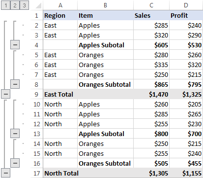
To create a nested (or inner) group, select all detail rows above the related summary row, and click the Group button.
For example, to create the Apples group within the East region, select rows 2 and 3, and hit Group. To make the Oranges group, select rows 5 through 7, and press the Group button again.
Similarly, we create nested groups for the North regions, and get the following result:
3. Add more grouping levels if necessary
In practice, datasets are seldom complete. If at some point more data is added to your worksheet, you will probably want to create more outline levels.
As an example, let's insert the Grand total row in our table, and then add the outermost outline level. To have it done, select all the rows except for the Grand Total row (rows 2 through 17), and click Data tab > Group button > Rows.
As shown in the screenshot below, our data is now grouped in 4 levels:
- Level 1: Grand total
- Level 2: Region totals
- Level 3: Item subtotals
- Level 4: Detail rows

Now that we have an outline of rows, let's see how it makes our data easier to view.
How to collapse rows in Excel
One of the most useful features of Excel grouping is the ability to hide and show the detail rows for a particular group as well as to collapse or expand the entire outline to a certain level in a mouse click.
Collapse rows within a group
To collapse the rows in a particular group, just click the minus button ![]() at the bottom of that group's bar.
at the bottom of that group's bar.
For example, this is how you can quickly hide all detail rows for the East region, including subtotals, and show only the East Total row:
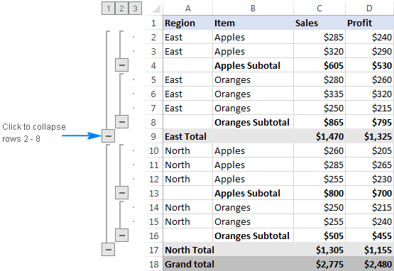
Another way to collapse rows in Excel is to select any cell in the group and click the Hide Detail button on the Data tab, in the Outline group:

Either way, the group will be minimized to the summary row, and all of the detail rows will be hidden.
Collapse or expand the entire outline to a specific level
To minimize or expand all the groups at a particular level, click the corresponding outline number at the top left corner of your worksheet.
Level 1 displays the least amount of data while the highest number expands all the rows. For example, if your outline has 3 levels, you click number 2 to hide the 3rd level (detail rows) while displaying the other two levels (summary rows).
In our sample dataset, we have 4 outline levels, which work this way:
- Level 1 shows only Grand total (row 18 ) and hides all other rows.
- Level 2 displays Grand total and Region subtotals (rows 9, 17 and 18).
- Level 3 displays Grand total, Region and Item subtotals (rows 4, 8, 9, 18, 13, 16, 17 and 18).
- Level 4 shows all the rows.
The following screenshot demonstrates the outline collapsed to level 3.

How to expand rows in Excel
To expand the rows within a certain group, click any cell in the visible summary row, and then click the Show Detail button on the Data tab, in the Outline group:

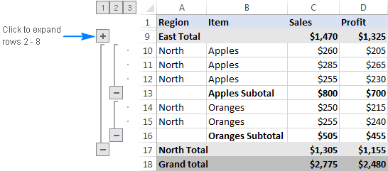
Or click the plus sign ![]() for the collapsed group of rows that you want to expand:
for the collapsed group of rows that you want to expand:
How to remove outline in Excel
In case you want to remove all row groups at once, then clear the outline. If you want to remove just some of the row groups (e.g. nested groups), then ungroup the selected rows.
How to remove the entire outline
Go to the Data tab > Outline group, click the arrow under Ungroup, and then click Clear Outline.

Notes:
- Removing outline in Excel does not delete any data.
- If you remove an outline with some collapsed rows, those rows might remain hidden after the outline is cleared. To display the rows, use any of the methods described in How to unhide rows in Excel.
- Once the outline is removed, you won't be able to get it back by clicking the Undo button or pressing the Undo shortcut (Ctrl + Z). You will have to recreate the outline from scratch.
How to ungroup a certain group of rows
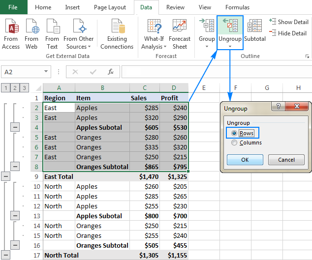
To remove grouping for certain rows without deleting the whole outline, do the following:
- Select the rows you want to ungroup.
- Go to the Data tab > Outline group, and click the Ungroup button. Or press Shift + Alt + Left Arrow which is the Ungroup shortcut in Excel.
- In the Ungroup dialog box, select Rows and click OK.
For example, here's how you can ungroup two nested row groups (Apples Subtotal and Oranges Subtotal) while keeping the outer East Total group:
Tips and notes:
- It is not possible to ungroup non-adjacent groups of rows at a time. You will have to repeat the above steps for each group individually.
- In Excel 365, you can use the GROUPBY function to group rows and aggregate values with a formula.
Excel grouping tips
As you have just seen, it's pretty easy to group rows in Excel. Below you will find a few useful tricks that will make your work with groups even easier.
How to calculate group subtotals automatically
In all of the above examples, we have inserted our own subtotal rows with SUM formulas. To have subtotals calculated automatically, use the Subtotal command with the summary function of your choice such as SUM, COUNT, AVERAGE, MIN, MAX, etc. The Subtotal command will not only insert summary rows but also create an outline with collapsible and expandable rows, thus completing two tasks at once!
Apply default Excel styles to summary rows
Microsoft Excel has the predefined styles for two levels of summary rows: RowLevel_1 (bold) and RowLevel_2 (italic). You can apply these styles before or after grouping rows.
To automatically apply Excel styles to a new outline, go to the Data tab > Outline group, click the Outline dialog box launcher, and then select the Automatic styles check box, and click OK. After that you create an outline as usual.
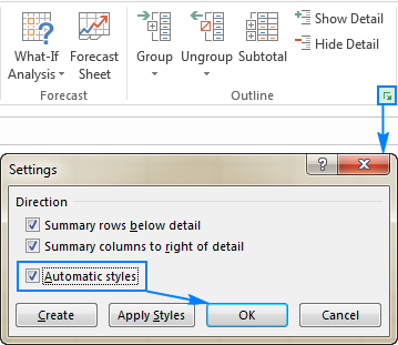
To apply styles to an existing outline, you also select the Automatic styles box as shown above, but click the Apply Styles button instead of OK.
Here's how an Excel outline with the default styles for summary rows looks like:

How to select and copy only visible rows
After you've collapsed irrelevant rows, you may want to copy the displayed relevant data somewhere else. However, when you select the visible rows in the usual way using the mouse, you are actually selecting the hidden rows as well.
To select only the visible rows, you'll need to perform a few extra steps:
- Select visible rows using the mouse.
For example, we have collapsed all of the detail rows, and now select the visible summary rows:

- Head to the Home tab >Editing group, and click Find & Select > Go To Special. Or press Ctrl + G (Go To shortcut) and click the Special… button.
- In the Go To Special dialog box, select Visible cells only and click OK.

As the result, only the visible rows are selected (the rows adjacent to hidden rows are marked with a white border):

And now, you simply press Ctrl + C to copy the selected rows and Ctrl + V to paste them wherever you like.
How to hide and show outline symbols
To hide or display the outline bars and level numbers in Excel, use the following keyboard shortcut: Ctrl + 8.
Pressing the shortcut for the first time hides the outline symbols, pressing it again redisplays the outline.
The outline symbols don't show up in Excel
If you can see neither the plus and minus symbols in the group bars nor the numbers at the top of the outline, check the following setting in your Excel:
- Go to the File tab > Options > Advanced category.
- Scroll down to the Display options for this worksheet section, select the worksheet of interest, and make sure the Show outline symbols if an outline is applied box is selected.

This is how you group rows in Excel to collapse or expand certain sections of your dataset. In a similar fashion, you can group columns in your worksheets. I thank you for reading and hope to see you on our blog next week.
 by
by
56 comments
When the data is formatted as a table in excel I can group the rows, however, I can't adjust it so the summary row is above the detail.
I appreciate one would ordinarily go to the Data tab > Outline group, click the Outline dialog box launcher, and then uncheck "Summary rows below detail", however, when the information is formatted as a table it wont let me click the Outline dialog box launcher.
Has anyone else experienced this and do you know how to make the summary row above detail (without having to convert the data back to a range rather than a table)?
Thanks
I have exactly the same issue. No summary rows, but a change in data type wants me to have summaries created above.
Cannot find help anywhere.
Hi! Unfortunately, these features are not available in Excel Table.
Hi, this should be a really easy question and I am embarrassed I cannot figure it out. I have 10 rows. All I want to do is create a grouping for the first 5 rows (row 1-5) and then create another grouping for the second set of 5 rows (row 6-10). I create the first grouping and it works fine. But when I select the rows 6-10 and click group, Excel combines all 10 rows into one group. Now there is only one group, and it either shows all 10 rows or nothing. But I want to be able to show either the first 5 rows or the last 5 rows. How do I accomplish that? Why does Excel combine all rows into one group even though I am selecting different rows (no overlap between the rows)?
Hi! If you add Subtotals to the first group of rows 1-5, the next rows 6-10 will be added to the new group.
below is my text string in Cell A1 & A2 we need to find the text "IN" in same cell two different place at a time & extract number showing before that text e. g. 193 & 62 (left side of text ) using if error formula.
TX01 INR 193IN TX02 INR 428K3 TX03 INR 236P2
TX01 INR 160YR TX02 INR 180YR TX03 INR 62IN
Hi! To extract numbers from text by pattern, use regular expressions and the RegExpExtract function. For more information, please visit: How to extract substrings in Excel using regular expressions (Regex).
=REPLACE(RegExpExtract(A1, "(\d+)IN"),LEN(RegExpExtract(A1, "(\d+)IN"))-1,2,"")
provide us for excel formulas below is not working.
=REPLACE(RegExpExtract(A1, "(\d+)IN"),LEN(RegExpExtract(A1, "(\d+)IN"))-1,2,"")
Dear Sir/Madam,
Below is my two text string in different formats, we need to find text "IN" only in mentioned strings and extract the number showing before that text e.g. 531 or 413 "IN" text place is not fix in string its randomly change any place using IFERROR formula if not found then return should be zero.
assuming below string in cell A1 and answer required in B2 = 531 or 413
INR 80-YR XT INR 531-IN INR 1835-K3 INR 236-P2
XT INR 413-IN INR 280-K3 INR 236-P2
Hi! Have you read the manual that was recommended to you? Add "-" to the formula
=REPLACE(RegExpExtract(A1, "(\d+)-IN"),LEN(RegExpExtract(A1, "(\d+)-IN"))-1,2,"")
I recommended you a guide. Follow the recommendations, install the function code in your workbook.
Hi…
I have a tool that produces a report listing files on a UNC path not accessed for some time, report can be 1000’s of lines
Eg 1 Row
\\server.com\sharename\folder1\folder2\spreadsheet. xlsx
What id like to do is automatically group the report at each folder level
The output from Treesize does this, but I don’t know how to do it from scratch in Excel
Hello, pls help me find a way to do this method of grouping....
in which we can expand or collapse data just like a drop down list, but instead of choosing a sigle data from dropdown list, i will be able to expand that cell with all the rows of data it hides.
i.e
similar to grouping but instead of the "+" and "-" symbols being shown outside the cells (in the left margin) in case of grouping, here the symbols will be on the cell itself which acts as a heading to the group of rows or data it contains or hides. so that when we press the "+" symbol it expands and "-" symbol it hides the data below just like when grouped.
A difference i wish to see by doing so (when compared to grouping) being that, i can filter the cells by hiding the inside contents and after filtering or sorting, i can expand without any loss of data within each such cells.
Hello! I'm trying to figure out how to group rows, but so that when filtering, Excel considers the grouped rows together and just uses the first data point in the group as the filter reference.
Does this make sense?
Did you ever figure this out? I'm trying to do the same thing.
Same question: once rows are grouped, I would then like to apply filters but keep the grouped rows together
Hi!
I can't change how Excel works. I can give you advice on how to write the formula.
Hi,
Thanks for the tips.
I'm using outline group and I'm trying to print just the active pages, but the hides one is print as blank. For example the sheets as 3 pgs when I use group reduce to 2 pgs, but it will print 3 with a blank pg in the middle.
Is there a simple way of getting that?
I know I could manually select the cells and print select area, but a lot of people use the file and I would like to be ready to go.
thank you advance
It is explained in the head of:
"How to select and copy only visible rows"
After following it, select all and paste in another Sheet of Excel. Print that sheet blank will be avoided
where can i get the sample dataset for practice.
Hi!
This was very helpful and easy to understand. I have seen it used before, but I didn't have a need for it myself until recently.
Side note:
I read some of the comments. My best advice for anyone with formatting or analysis questions is to start using Tables and Power Query. I held out on PQ for so long thinking the learning curve was too high and it wouldn't be useful for my needs. I'm still just getting started and I can already admit I was wrong.
Now I just need to convince my coworkers to stop sending me .xls files...
It's 2022 and I'm still finding this site - and this page in particular - super useful. Thank you!
I have an excel database of approximately 204,000, with about 15,000 different names. Each name is repeated identically multiple times, depending upon how long they were current (in alphabetical order).
I would like each name under the heading 'student ID' to be regarded as a separate group, and tell it to select the “last row in each student id group”. The aim being to end up with just one record for each of the approximately 15,000 students.
Is this possible, and if so how do I achieve it?
Hi!
I don't really understand what you want to do. This article explains how to group rows in Excel. If you didn't find the information you wanted, please describe the problem in more detail.
I am building a spreadsheet that functions like a gantt chart (manually), so there are no calculations. I would like to show the client, project, and deadline on one row (I'll call it the header row). Below that, I would like to list tasks and corresponding start/end dates for that project. This will continue with various clients and projects.
So, I would like to know if there is a way to group the header row and all subsequent task rows so that I can keep them together when sorting? For example, I may want to sort by client, project, or deadline (based on the header row) and be sure that all task rows stay grouped with the header row.
If this is possible, is there also a way to collapse the task rows or hide them from view?
Hello!
I don't know what your datasheet looks like. But you may find the Excel Advanced Filter tool useful.
How can I post a EXCEL sheet as an example to ask the question to you and get solution from you.
I am using cut and paste below to send you sheet in case I can not attach the sheet. I want to add numbers in a column & show addition in the row next to last row in the column.
Thanking you. RAKESH
98,000.00 98,000.00 1,33,298.00 2,70,000.00 2,70,000.00 2,70,000.00
3,50,000.00 3,50,000.00 4,76,065.00 2,14,000.00 2,14,000.00 2,14,000.00
Hi , when I create a Create nested groups (level 2) it ungroup my last sub group is so annoying . Why ?
We have a gsheet that is shared with three colleagues. They could not collapse grouped ones. Is there a way to give them access to it too?
Awesome. Its really helpful
Hi,
I would like to auto/update grouped rows in pivot table when rows are added/removed from the data source rather than manually regrouping. Could anyone help with this?
Thanks in advance.
Hi!
I want to create a PR plan and use grouping for activities related to the same main activity, but run to problems. I want to group 2-10 rows leaving the first row visible to mark the main activiti.
For example my activity item is an article published on my website and have 5 items related to it. Now if I group all of these 6 rows, they all collide and hide. I can leave the first row ungrouped, but that wouldn't be the point of grouping.
And if I have only 2 activites, then it wouldn't make any sense to group 1 row and leave one row visible.
So long story short: how can I group rows in a way that would leave the first row visible?
Is there a way to move the (+) symbol in line with the row the subset of data corresponds to? Excel is automatically placing the symbol one row down.
Alt, A, L; This opens the settings menu. Then make sure to uncheck the "Summary rows before detail" box.
Hi - This is useful but does not help with my much simpler problem. I will use a simple example to explain my problem
Column A is School
Column B is Student
So there will be multiple occurrences of the same School value on consecutive rows for each student
I would like to be able to group by School automatically so as to be able to expand/collapse School to reveal and collapse to show all students. I have no wish to sum anything, this is purely to make the sheet manageable
Any ideas - this seems like it should be simple