In this article I'll show you 3 ways how you can add hyperlinks into your Excel workbook to easily navigate between numerous worksheets. You'll also learn how to change a link destination and modify its format. If you don't need a hyperlink any more, you'll see how to quickly remove it.
If you are a real Internet surfer, you know firsthand about the bright sides of hyperlinks. Clicking on hyperlinks you instantly get access to other information no matter where it is located. But do you know the benefits of spreadsheet hyperlinks in Excel workbooks? The time has come to discover them and start using this great Excel feature.
One of the ways you can put spreadsheet hyperlinks to good use is to create a table of contents of your workbook. Excel internal hyperlinks will help you to quickly jump to the necessary part of the workbook without hunting through multiple worksheets.
Insert a hyperlink in Excel
If you need to add a hyperlink in Excel 2016 or 2013, you can choose one of the following hyperlink types: a link to an existing or new file, to a web page or e-mail address. Since the subject of this article is creating a hyperlink to another worksheet in the same workbook, below you'll find out three ways to do that.
Add a hyperlink from the context menu
The first method of creating a hyperlink within one workbook is to use the Hyperlink command.
- Select a cell where you want to insert a hyperlink.
- Right-click on the cell and choose the Hyperlink option from the context menu.
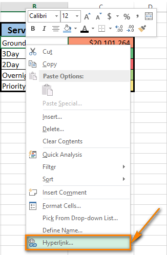
The Insert Hyperlink dialog window appears on the screen. - Choose Place in This Document in the Link to section if your task is to link the cell to a specific location in the same workbook.
- Select the worksheet that you want to link to in the Or select a place in this document field.
- Enter the cell address in the Type the cell reference box if you want to link to a certain cell of another worksheet.
- Enter a value or name into the Text to display box to represent the hyperlink in the cell.
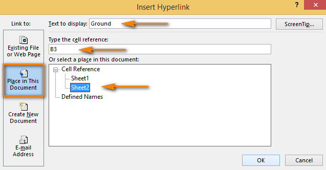
- Click OK.

The cell content becomes underlined and highlighted in blue. It means that the cell contains the hyperlink. To check if the link works, just hover the pointer over the underlined text and click on it to go to the specified location.
Excel HYPERLINK function
Excel has a HYPERLINK function that you can also use for creating links between spreadsheets in the workbook. If you are not good at entering Excel formulas immediately in the Formula bar, do the following:
- Select the cell to which you want to add a hyperlink.
- Go to Function Library on the FORMULAS tab.
- Open the Lookup & Reference drop-down list and choose HYPERLINK.
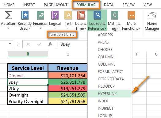
Now you can see the function name in the Formula bar. Just enter the following two HYPERLINK function arguments in the dialog window: link_location and friendly_name.
In our case link_location refers to a specific cell in another Excel worksheet and friendly_name is the jump text to display in the cell.
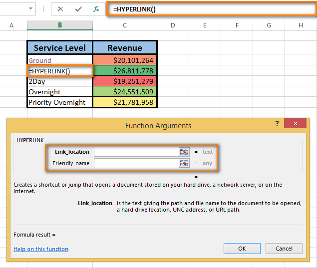
Note. It's not a must to enter friendly_name. But if you want the hyperlink to look neat and clear, I'd recommend to do it. If you don't type in friendly_name, the cell will display the link_location as the jump text.
- Fill in the Link_location text box.

Tip. If you don't know what address to enter, just use the Select range icon to pick the destination cell.
The address displays in the Link_location text box.

- Add the number sign (#) before the specified location.
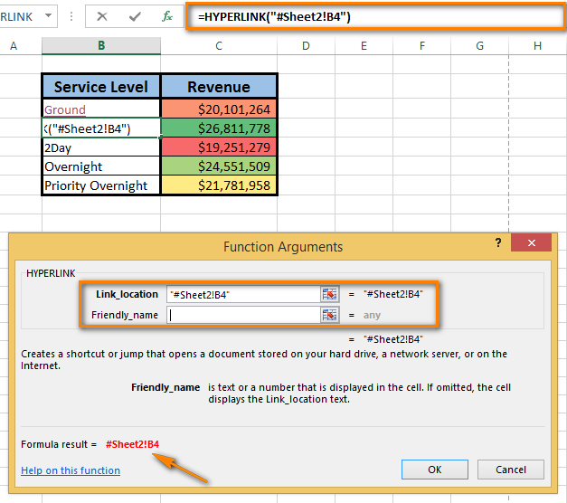
Note. It is crucial to type the number sign. It indicates that the location is within the current workbook. If you forget to enter it, the link won't work and an error will appear when you click on it.
When you move to the Friendly_name text box, you see the formula result in the bottom-left corner of the Function Arguments dialog.
- Enter Friendly_name that you want to display in the cell.
- Click OK.
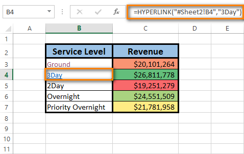
Here you are! Everything is as it should be: the formula is in the Formula bar, the link is in the cell. Click on the link to check where it follows.
Insert a link by cell drag-and-drop
The quickest way of creating hyperlinks within one workbook is using the drag-and-drop technique. Let me show you how it works.
As an example, I'll take a workbook of two sheets and create a hyperlink in Sheet 1 to a cell in Sheet 2.
Note. Make sure that the workbook is saved because this method doesn't work in new workbooks.
- Select the hyperlink destination cell in Sheet 2.
- Point to one of the cell borders and right-click.

- Hold the button and go down to the sheet tabs.

- Press the Alt key and mouse over the Sheet 1 tab.
Having the Alt key pressed automatically takes you to the other sheet. Once Sheet 1 is activated, you can stop holding the key. - Keep dragging to the place where you want to insert a hyperlink.
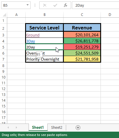
- Release the right mouse button for the popup menu to appear.
- Choose Create Hyperlink Here from the menu.

After you do that, the hyperlink appears in the cell. When you click on it, you'll switch to the destination cell in Sheet 2.
No doubt that dragging is the fastest way to insert a hyperlink into an Excel worksheet. It combines several operations into a single action. It takes you less time, but a bit more attention concentration than two other methods. So it's up to you which way
to go.
Edit a hyperlink
You can edit an existing hyperlink in your workbook by changing its destination, its appearance, or the text that is used to represent it.
Change link destination
As this article deals with hyperlinks between spreadsheets of the same workbook, the hyperlink destination in this case is a specific cell from another spreadsheet. If you want to change the hyperlink destination, you need to modify the cell reference or choose another sheet. You can do both, if necessary.
- Right-click the hyperlink you want to edit.
- Choose Edit Hyperlink from the popup menu.

The Edit Hyperlink dialog box appears on the screen. You see that it looks the same as the Insert Hyperlink dialog and has the identical fields and layout.

Note. There are, at least, two more ways to open the Edit Hyperlink dialog. You can press Ctrl + K or click on Hyperlink in the Links group on the INSERT tab. But don't forget to select the necessary cell before doing it.
- Update the information in the appropriate fields of the Edit Hyperlink dialog.
- Click OK and check where the hyperlink jumps to now.
Note. In case you used Method 2 to add a hyperlink in Excel, you need to edit the formula to change the hyperlink destination. Select the cell that contains the link, and then place the cursor in the Formula bar to edit it.
Modify hyperlink format
Most of the time hyperlinks are shown as an underlined text of blue color. If the typical appearance of hyperlink text seems to you boring and you'd like to stand out of the crowd, go ahead and read below how to do it:
- Go to the Styles group on the HOME tab.
- Open the Cell Styles list.
- Right-click on Hyperlink to change the appearance of the hyperlink that was not clicked. Or right-click Followed Hyperlink if the hyperlink was activated.
- Choose the Modify option from the context menu.

- Click on Formatin the Styles dialog box.
- Make the necessary changes in the Format Cells dialog window. Here you can change the hyperlink alignment and font or add fill color.
- When you are done, click OK.
- Make sure that all the changes are marked under Style includes in the Style dialog box.
- Press OK.

Now you can enjoy a new individual style of the hyperlinks in your workbook. Pay attention that the changes you made affect all the hyperlinks in the current workbook. You can't change the appearance of a single hyperlink.
Remove a hyperlink
It will take you a few seconds and no efforts to delete a hyperlink from the worksheet.
- Right-click the hyperlink you want to remove.
- Choose the Remove Hyperlink option from the popup menu.
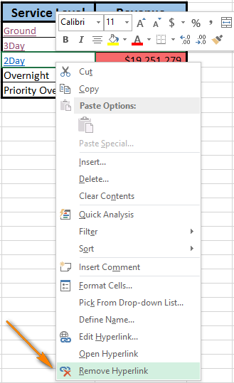
The text remains in the cell, but it is no longer a hyperlink.
Note. If you want to delete a hyperlink and the text that represents it, right-click the cell that contains the link and choose the Clear Contents option from the menu.
This trick helps you to delete a single hyperlink. If you want to know how to remove multiple (all) hyperlinks from Excel worksheets at a time, follow the link to our previous blog post.
I hope that in this article you saw the simplicity and effectiveness of using internal hyperlinks in a workbook. Just a few clicks to create, jump and discover the massive content of complex Excel documents.
 by
by
40 comments
Hello,
I have an Excel workbook with multiple sheets in it. The first sheet is a summary sheet, and I've added many hyperlinks to different cells in another sheet of the same workbook. However, when I sort or filter the summary sheet, the hyperlinks do not update accordingly. Now, when I now click on a hyperlink, it brings me to a different cell.
Is there anyway to make dynamic hyperlinks which update when sorting/filtering the first summary sheet?
Thanks for your help, much appreciated!
Hello Chris!
You can create dynamic hyperlinks in Excel that update automatically when sorting or filtering the first summary sheet.
This approach uses the HYPERLINK function combined with INDEX MATCH functions to create a dynamic hyperlink that updates based on your sorting or filtering actions. Here’s how you can do it:
Select the cell where you want to create the hyperlink.
Use the following formula in the formula bar:
=HYPERLINK("#'"&SheetName&"'!"&CELL("address",INDEX(SheetName!A1:A10, MATCH(lookup_value, SheetName!A1:A10, 0))),"Link Text")
Replace "SheetName" with the name of your sheet, "lookup_value" with the value you're matching, and "Link Text" with the text you want to display as the hyperlink.
Ensure that the lookup_value and SheetName are dynamic, so when you sort or filter the sheet, the hyperlink updates accordingly.
For the detailed instructions, please see: How to use Excel HYPERLINK function to create different link types.
Hi,
Hope someone could help with this hyperlink query.
I have one workbook and two sheets; Sheet 1 named Upload, Sheet 2 named Approval. On sheet 1, I have a column with numbers 1-10 which on each number I have inserted a hyperlink with an invoice to it and if you click on the rows 1-10 a pfd will open up with an invoice attached.
I want to be able to go to sheet 2 and create a column with number 1-10 and i want to have the same invoices hyperlinked so each number mirrors work sheet 1 upload. How can I get this hyperlink function to work on Sheet 2 Approval without having to do the steps of hyperlinking all over again.
I hope someone can assist with these as i have been researching and trying for days now and i can't seem to get it to work.
Many thanks
Arina
Hello Arina!
Try to simply copy and paste the cells together with the hyperlinks. You can also use the HYPERLINK function. Read more: Excel HYPERLINK function to quickly create and edit multiple links. I hope it’ll be helpful.
We have spreadsheet with close to 40 tabs. Teh names of those tabs are in column A. I would like to use that column A reference to create the hyperlink based on the value in column A. Is this possible?
Hi! If I understand you correctly, you can use the HYPERLINK function to create a hyperlink based on a cell value. Try to follow the recommendations from this article: How to use Excel HYPERLINK function to create different link types
how to link a cell from one sheet to all other sheets in the same workbook ? For Example on Sheet 1 in Cell A1 and A2 I have data, the same data should flow on rest all of the sheets in the workbook. Do we have any formulas ?
An Excel formula cannot transfer data to another cell. It can get data from another cell. So on each worksheet, write a formula that will get data from that cell A1. It will be a regular Excel cell reference. Read more: Excel reference to another sheet or workbook (external reference). You can transfer data to other cells on other worksheets using a VBA macro.
Hi, I have a query.
I have a summary sheet (Summary) and four different assessment templates as different sheets (SheetA, SheetB, SheetC, SheetD)
In summary sheet there will be a formula in Column D of each row (D3, D4, D5, D6, D7....D50) which Assessment sheet to be used.
Based on the inputs in Column A, B, C, value will appear in Column D as " Use Sheet B" or "Use Sheet D" or "Use Sheet A".
Now how to link the result in Column D of summary sheet into respective Assessment sheets?
Please help on this.
Hi! You can create a dynamic reference using the INDIRECT function. The following tutorial should help: INDIRECT formula to dynamically refer to another worksheet.
i want to link cell to cell in same sheet can you help me. example i want to click one cell and cell go to another cell linked with other.
Hi!
Here is the article that may be helpful to you: Hyperlink in Excel: how to create, edit and remove.
I want a hyperlink to send me to another sheet which then will linkbyo a drop down list that will match the name on the oth page.. is this possible?
Hi!
If I understand correctly, you can hyperlink to a cell with a drop-down list. Read more here: Hyperlink in Excel: how to create, edit and remove.
I want to create a hyperlink which contains a jump to another sheet in the same workbook. The name of the sheet shall not be "hard coded" but taken from a cell. For illustration:
- cell B4 contains "Sheet14", which is the name of a sheet
- desired hyperlink: =hyperlink (...B4...!A1;"Jump to sheet")
Hello!
I believe the following formula will help you solve your task:
=HYPERLINK("#"&B4&"!A1","Jump to sheet")
Great, this works - thank you!
Can any one help
I have two sheets A and B
Sheet A is for user
Sheet B for email
I have hyperlink "mailto:" on sheetB Cell B6 and I have hide this sheet , now on SheetA Cell A2 I want to create link with hided sheet's cell B6
whenever I click on A2 it work like I clicked on B6 .
How can I link with A2 to B6
Hello!
If I understood your question correctly, create a external reference to a cell in another worksheet, and then you can hide that sheet. You can also just write a link to a cell using the F2 key to edit it.
Hello,
I have an Excel workbook with several sheets in it - the first sheet is a summary sheet listing each employee, and then every employee has an individual sheet. I have set up hyperlinks between the each worksheet and the summary sheet for easy navigation backwards and forwards.
However, when I add a new employee row in the summary sheet, the hyperlinks do not update on the individual employee sheets, therefore when I now click on 'Joe Bloggs'' hyperlink, to return to the summary sheet, it brings me to the row above/below that reference.
So my question is, is there anyway to make dynamic hyperlinks which would update when a new row is added into that first summary sheet?
Thanks for your help, all advice appreciated.
Hello!
You can create dynamic hyperlinks using the MATCH function.
The formula for a dynamic hyperlink could look like this:
=HYPERLINK("#"&"SummarySheet!B"&(MATCH(B2, SummarySheet!$B$3:$B$100,0)+2),"Click Here to See Data")
where:
B2 - employee name
The # sigh indicates the formula to refer to the same workbook.
SummarySheet!B - is a reference to the sheet name and column name in the symmary table.
MATCH(B2, SummarySheet!$B$3:$B$100,0) returns the position of the corresponding employee in the summary sheet. 2 is added to it because the data list starts on the third row.
I hope my advice will help you solve your task.
Thanks so much Alexander.
I have entered the following formula: =HYPERLINK("#"&"EE''s!''&(MATCH(B10,EE''s'!$B$6:$B$500,0)+6),""Click Here to See Data")
My Employee's worksheet is named EE's and the Employee Name is in cell B10. The list of names start in cell B6. When I click on hyperlink, I'm getting an error message to say that the reference isn't valid. Have I missed something?
Thanks for your help, I appreciate it.
Dawn
Hi!
If the worksheet name includes spaces or non-alphabetical characters, you must enclose it in single quotation marks. For more information, please visit: How to reference another sheet in Excel.
Is there a way to click a cell/hyperlink on sheet 1 which takes you to a filtered list on sheet 2 within the same workbook.
Ive seen people writing code o do this but its beyond my skill level.
Hello!
Perhaps this instruction will be useful to you: Hyperlink to a sheet or cell in the current workbook.
in column A i have the heading ITEM, column B the heading COST and in column C the heading PROFIT. in column G (in the same sheet) i just want to type the ITEM and it must display the ITEM and the COST and the PROFIT. is it possible for you to HELP PLEASE?(each heading must display in its own cell)
Hello!
Please have a look at this article: Vlookup to return multiple matches in rows.
I hope my advice will help you solve your task.
I am certain I am not the only person with this question, so hopefully it can be answered easily?
I have varying reports that are compared at different intervals but all cross-reference each other. i.e., budget projections reports v actuals, receivables v outstanding etc.
So when a comparison needs to be set up, can spreadsheet cells across varying workbooks/documents be hyperlinked into one spreadsheet/workbook to produce 'differences/results' reporting?
Hope that's a clear question!? I apologize if its confusing - but I've been out of work 20 years and I'm trying to refresh all my OLD accounting skills used in much earlier versions of the software!
Thank you!
Hello!
External references are used to link spreadsheet cells in different workbooks. I also recommend paying attention to pivot tables.
Thank you so much! This information saved my bacon!
Please say me solution
Can you hyperlink from one cell in one document to another cell in a separate document? Basically, I want to be able to click on a cell and it open the other document at the same place.
Nothing I have tried has worked.
When I use the first method to create HYPERLINK to another sheet, it says "cannot open the file specified".
Little help here.. :)
Justin, make sure you put in the # before the sheet name. I suspect your error is related to this omission on your formula.
Hello, is there a way for the selected cell to go to the top of the page? Currently the hyperlink goes to a cell like A124 and that is displayed at the bottom of the page. How can I create a hyperlink that will go to that page and display A124 at the top of the page? Any assistance would be greatly appreciated!
Yes, tell it to go to A1, insetad of A124. Right click, edit and the second box is the cell that you want it to reference.
but what if I insert a row before the destination cell? will the hyperlink self adjust to continue pointing to the originally intended destination cell, or would I need to manually adjust the hyperlink to point to the new destination?
Please, someone, answer Chris' enquiry, as I need to know the answer too. And if possible a method of auto-updating the link, if possible. (in Excel 2019)
Hello!
Unfortunately, the hyperlink formula cannot keep track of any changes that occur on the target sheet.