This article will guide you on how to use LARGE function in Excel with many formula examples.
When analyzing a set of numbers, it often makes sense to find the biggest ones. Getting the highest value is super-easy with the MAX function. When it comes to targeting a specific largest value, say the 2nd or the 3rd biggest number in a dataset, the LARGE function comes in handy.
Excel LARGE function
The LARGE function in Excel is used to return the n-th largest value from a numeric data set. For example, it can calculate the highest score, the 2nd largest order, the 3rd place result, and so on.
The syntax consists of two argument, both of which are required:
Where:
- Array - a range or an array where to search for the largest value.
- K - the position from the highest to return, i.e. k-th largest value in a dataset.
LARGE is categorized under Statistical functions. It is available in all versions of Excel for Office 365, Excel 2021, Excel 2019, Excel 2016, Excel 2013, Excel 2010, and earlier.
3 things to know about LARGE function
Before we get to more practical things and start building our own formulas, please pay attention to 3 simple facts that explain the essentials:
- The LARGE function processes only numeric values. Blank cells, text, and logical values are ignored.
- If array contains any errors, an error is returned.
- In case array contains n values, LARGE(array,1) will return the maximin value, and LARGE(array,n) will return the minimum value.
Basic LARGE formula
In its basic form, a LARGE formula in Excel is very easy to build. For the 1st argument, you supply a range of numeric values. In the 2nd argument, you define the position from largest to return.
In the sample table below, supposing you wish to know the 2nd largest score. This can be done with the following formula:
=LARGE(B2:B10, 2)
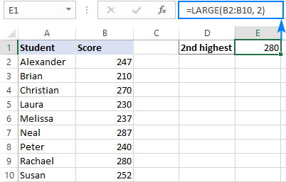
How to use LARGE formula in Excel - examples
And now, let's look at more specific use cases and see how the LARGE function could be helpful.
How to get top N values in Excel
To get the largest 3, 5, 10, etc. values with a single formula, carry out these steps:
- Type the positions of interest in separate cells. These numbers will be used as k values.
- Make a LARGE formula applying an absolute range reference for array ($B$2:$B$10 in our case) and relative cell reference for k (D3).
- Enter the formula in the topmost cell, and then drag it down to the below cells. Done!
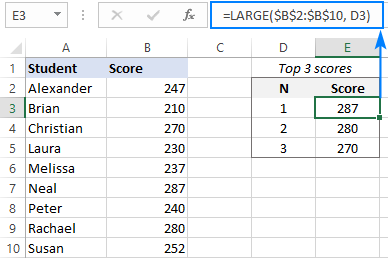
As an example, we are going to find the top 3 scores in the table below. For this, we type the numbers 1, 2 and 3 in D3, D4 and D5, respectively, and enter the following formula in E3:
=LARGE($B$2:$B$10, D3)
Drag it through E4, and you will get this result:
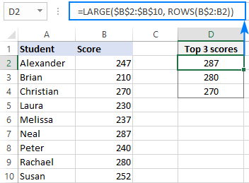
Instead of typing the positions on the sheet, you can use the ROWS function with an expanding range reference to generate the k values automatically as explained in Excel formula to find top N values in a list.
=LARGE($B$2:$B$10, ROWS(B$2:B2))
Tip. You can also use the LARGE function to extract top N records with advanced filter.
How to sum or average largest N values
To sum top n values in a data set, you can use LARGE together with either SUMPRODUCT or SUM in this way:
Or
To average the highest n values, combine the AVERAGE and LARGE functions:
To see how it works in practice, let's find an average of the top 3 scores in our sample table. For this, we are using this formula:
=AVERAGE(LARGE(B2:B10, {1,2,3}))
To add up the highest 3 scores, the formula is:
=SUM(LARGE(B2:B10, {1,2,3}))
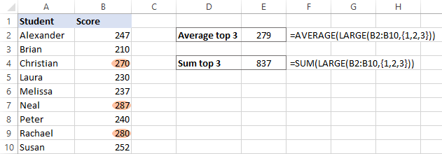
Note. In case you use a range rather than an array constant for k, you need to press Ctrl + Shift + Enter to make it an array formula. In Excel 365 that supports dynamic arrays, all formulas can be completed as usual by pressing the Enter key.
How these formulas work:
Normally, the LARGE function returns a single value based on the k number. In these formulas, we supply an array constant like {1,2,3} for the k argument forcing it to return an array of values. That array goes to the outer function to be summed or averaged.
Get data associated with the n-th largest value
To retrieve information relating to the largest values, just nest the LARGE function in the canonical INDEX MATCH formula:
Where:
- Return_array is a range from which to extract matches.
- Lookup_array is a range of numbers to rank from highest.
- N is the position of the largest value to search for.
For example, to get the name of a student who did best on the exams, nter this formula in F3:
=INDEX($A$2:$A$10, MATCH(LARGE($B$2:$B$10, $D3), $B$2:$B$10, 0))
Where A2:A10 is the return array (names), B2:B10 is the lookup array (scores) and D3 is the position from largest.
To find out who has the 2nd and 3rd highest scores, copy the forma to F4 and F5:
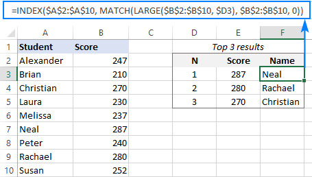
Notes:
- This solution works nice for unique values. If your dataset contains duplicate numbers, "ties" in ranking may occur, which will produce incorrect results. To prevent this from happening, use a more complex formula to handle ties.
- In Excel 365, you can use new dynamic array functions to work out a much simpler solution that resolves a problem of ties automatically. For full details, please see How to filter top N values in Excel.
LARGE formula to sort numbers descending
To quickly sort a list of numbers in Excel 365, you can use the new SORT function. In Excel 2019, 2016 and earlier versions that do not support dynamic arrays, we have to rely on the good old LARGE function to sort descending and SMALL to sort ascending.
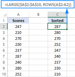
For this example, we will sort numbers in A2:A10 from highest to lowest. To have it done, we'll again need the ROWS function with an expanding range reference to increment the k argument by 1 with every row:
=LARGE($A$2:$A$10, ROWS(A$2:A2))
The above formula goes to the topmost cell (C2). And then, you drag it through as many cells as there are numbers in the original list (C2:C10 in our case):
LARGE formula for dates and times
As you know, dates and times in Excel are numeric values: dates are stored as integers and times as decimals. What does that mean for us? The LARGE function calculates date and time values in exactly the same way as it does numbers. In other words, the formula you used for numbers will work for dates and times too!
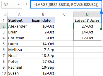
Assuming you have a list of dates in B2:B10, the following formula will return the most recent N dates, depending on how many cells you copy it to:
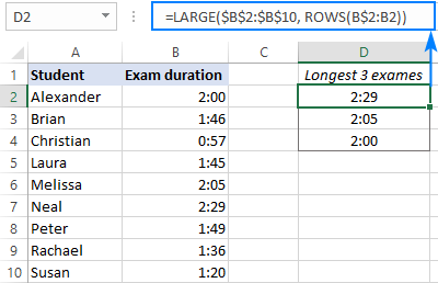
=LARGE($B$2:$B$10, ROWS(B$2:B2))
The same formula can also find the longest 3 times:
Get a future date closest to today or specified date
This example shows a more specific usage of the Excel LARGE function with dates.
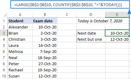
From a list of dates in B2:B10, suppose you wish to return a future date closest to today. To accomplish the task, we'll use the COUNTIF and TODAY functions together to calculate a value for the k argument of LARGE:
=LARGE($B$2:$B$10, COUNTIF($B$2:$B$10, ">"&TODAY()))
To find the next but one date, the formula is:
=LARGE($B$2:$B$10, COUNTIF($B$2:$B$10, ">"&TODAY())-1)
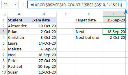
To find a date that comes right after a given date, input the target date in some cell (E3 in this example), and concatenate that cell reference in COUNTIF's criteria:
=LARGE($B$2:$B$10, COUNTIF($B$2:$B$10, ">"&E1))
In situation when a date matching your criteria is not found, you can use the IFERROR function as a "wrapper" to catch an error and replace it with whatever text you see fit:
=IFERROR(LARGE($B$2:$B$10, COUNTIF($B$2:$B$10, ">"&E1)), "Not found")
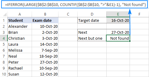
How this formula works:
In essence, you use the COUNTIF function to count how many dates in the list are greater than today or a specified date. That count is the k value the LARGE function needs.
At the moment of writing, today's date was October 7, 2020. The COUNTIF function with ">"&TODAY() for criteria determined that in B2:B10 there are 4 dates greater than 7-Oct-2020. Meaning, the 4th largest date in the list is the closest future date we are looking for. So, we plug COUNTIF into the 2nd argument of LARGE and get the desired result:
=LARGE($B$2:$B$10, 4)
The next but one date is the 3rd largest date in our case. To get it, we subtract 1 from COUNTIF's result.
Excel LARGE function not working
A LARGE formula may throw a #NUM! error because of the following reasons:
- The supplied array is empty or does not contain a single numeric value.
- The k value is a negative number.
- The k value is greater than the number of values in array.
That's how to use the LARGE function in Excel to find highest values in a dataset. I thank you for reading and hope to see you on our blog next week!
Practice workbook for download
Excel LARGE formula examples (.xlsx file)
 by
by
2 comments
Q: How to place position of a number from number list? Example there are % marks of several students in Class 12 exam in a table with their name. In last column, i want to put their place from this total group. i.e., 1, 2, 3, 4....n toppers
A: Try to follow the recommendations from this article: Excel RANK function and other ways to calculate rank.