The tutorial explains the basics of the modified internal rate of return, in what way it is different from IRR, and how to calculate MIRR in Excel.
For many years, finance experts and textbooks have warned about the flaws and deficiencies of the internal rate of return, but many executives keep using it for assessing capital projects. Do they enjoy living on the edge or simply are not aware of the existence of MIRR? Though not perfect, the modified internal rate of return resolves two main issues with IRR and provides a more realistic evaluation of a project. So, please meet the Excel MIRR function, which is our star guest today!
What is MIRR?
The modified internal rate of return (MIRR) is a financial metric to estimate the profitability of a project and rank equally sized investments. As its name suggests, MIRR is a modified version of the traditional internal rate of return that aims to overcome some deficiencies of IRR.
Technically, MIRR is the rate of return at which the net present value (NPV) of terminal inflows is equal to the investment (i.e. outflow); whereas IRR is the rate that makes the NPV zero.
IRR implies that all positive cash flows are reinvested at the project's own rate of return while MIRR allows you to specify a different reinvestment rate for future cash flows. For more information, please see MIRR vs. IRR.
How do you interpret the rate returned by MIRR? As with IRR, the bigger the better :) In situation when the modified internal rate of return is the only criterion, the decision rule is very simple: a project can be accepted if its MIRR is greater than the cost of capital (hurdle rate) and rejected if the rate is lower than the cost of capital.
Excel MIRR function
The MIRR function in Excel calculates the modified internal rate of return for a series of cash flows that occur at regular intervals.
The syntax of the MIRR function is as follows:
Where:
- Values (required) – an array or a range of cells that contains cash flows.
- Finance_rate (required) – the interest rate that is paid to finance the investment. In other words, it's the cost of borrowing in case of negative cash flows. Should be supplied as percentage or a corresponding decimal number.
- Reinvest_rate (required) – the compounding rate of return at which positive cash flows are reinvested. It is supplied as percentage or a decimal number.
The MIRR function is available in Excel for Office 365, Excel 2019, Excel 2016, Excel 2013, Excel 2010, and Excel 2007.
5 things you should know about MIRR in Excel
Before you go to calculate modified IRR in your Excel worksheets, here's a list of useful points to remember:
- The values must contain at least one positive (representing income) and one negative (representing outlay) number; otherwise a #DIV/0! error occurs.
- The Excel MIRR function assumes that all cash flows happen at regular time intervals and uses the order of values to determine the order of cash flows. So, be sure to enter the values in chronological order.
- It is implicitly implied that all cash flows happen at the end of a period.
- Only numeric values are processed. Text, logical values and empty cells are ignored; however, zero values are processed.
- A common approach is to use the weighted average cost of capital as the reinvest_rate, but you are free to input any reinvestment rate that you deem appropriate.
How to calculate MIRR in Excel – formula example
Calculating MIRR in Excel is very straightforward – you just put the cash flows, cost of borrowing and reinvestment rate in the corresponding arguments.
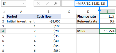
As an example, let's find the modified IRR for a series of cash flows in A2:A8, finance rate in D1, and reinvest rate in D2. The formula is as simple as this:
=MIRR(A2:A8,D1,D2)

Tip. If the result is displayed as a decimal number, set the Percentage format to the formula cell.
MIRR Excel template
To quickly evaluate different projects of unequal size, let us create a MIRR template. Here's how:
- For the cash flow values, make a dynamic defined range based on this formula:
=OFFSET(Sheet1!$A$2,0,0,COUNT(Sheet1!$A:$A),1)Where Sheet1 is the name of your worksheet and A2 is the initial investment (first cash flow).
Name the above formula as you like, say Values.
For the detailed steps, please see How to make a dynamic named range in Excel.
- Optionally, name the cells containing the finance and reinvest rates. To name a cell, you can use any of the methods described in How to define a name in Excel. Please note that naming these cells is optional, regular references will work as well.
- Supply the defined names you created to the MIRR formula.
For this example, I've created the following names:
- Values – the OFFSET formula described above
- Finance_rate – cell D1
- Reinvest_rate – cell D2
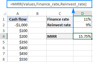
So, our MIRR formula takes this shape:
=MIRR(Values, Finance_rate, Reinvest_rate)
And now, you can type any number of values in column A, beginning in cell A2, and your MIRR calculator with a dynamic formula will immediately give a result:

Notes:
- For the Excel MIRR template to work correctly, the values must be input in adjacent cells without gaps.
- If the finance rate and reinvest rate cells are blank, Excel assumes they are equal to zero.
MIRR vs. IRR: which is better?
While the theoretical basis of MIRR is still disputed among finance academics, generally it is considered a more valid alternative to IRR. If you are not sure which method produces more accurate results, as a compromise you can calculate both, keeping in mind the following limitations.
IRR limitations
Though IRR is a commonly accepted measure of an investment's attractiveness, it has several inherent problems. And MIRR solves two of them:
1. Reinvestment rate
The Excel IRR function works under the assumption that interim cash flows are reinvested at the rate of return equal to the IRR itself. The catch is that in real life, firstly, a reinvestment rate tends to be lower than a finance rate and closer to the company's cost of capital and, secondly, the discount rate may change substantially over time. As the result, IRR often gives an overly optimistic view on the project's potential.
MIRR more accurately reflects the profitability of the investment because it considers both the finance and reinvest rate and allows you to change the anticipated rate of return from stage to stage in a long-term project.
2. Multiple solutions
In event of alternating positive and negative values (i.e. if a series of cash flows changes sign more than once), IRR can give multiple solutions for the same project, which leads to uncertainty and confusion. MIRR is designed to find only one value, eliminating the problem with multiple IRRs.
MIRR limitations
Some finance experts consider the rate of return produced by MIRR less reliable because a project's earnings are not always fully reinvested. However, you can easily make up for partial investments by adjusting the reinvest rate. For example, if you expect the reinvestments to earn 6%, but only half of the cash flows are likely to be reinvested, use the reinvest_rate of 3%.
MIRR function not working
If your Excel MIRR formula results in an error, there are the two main points to check:
- #DIV/0! error. Occurs if the values argument does not contain at least one negative and one positive value.
- #VALUE! error. Occurs if the finance_rate or reinvest_rate argument is non-numeric.
That's how to use MIRR in Excel to find the modified rate of return. For practice, you are welcome to download our sample workbook to Calculating MIRR in Excel. I thank you for reading and hope to see you on our blog next week!
 by
by