In this short tutorial, we'll talk about Excel SMALL function, how it works and how to use it to find the Nth smallest number, date, or time.
Need to find a few lowest numbers in a worksheet? This is quite easy to do with the Excel Sort feature. Do not want to waste time on re-sorting your data with every change? The SMALL function will help you quickly find the lowest value, second smallest, third smallest, and so on.
Excel SMALL function
SMALL is a statistical function that returns the n-th smallest value in a data set.
The syntax of the SMALL function includes two arguments, both of which are required.
SMALL(array, k)
Where:
- Array - an array or a range of cells from which to extract the smallest value.
- K - an integer that indicates the position from the lowest value to return, i.e. k-th smallest.
The function is available in all versions of Excel for Office 365, Excel 2021, Excel 2019, Excel 2016, Excel 2013, Excel 2010, and earlier.
Tip. To find k-th lowest value with criteria, use Excel SMALL IF formula.
Basic SMALL formula in Excel
A SMALL formula in its basic form is very easy to build - you just specify the range and the position from the smallest item to return.
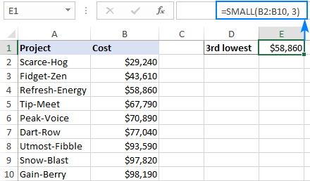
In the list of numbers in B2:B10, supposing you want to extract the 3rd smallest value. The formula is as simple as:
=SMALL(B2:B10, 3)
To make it easier for you to check the result, column B is sorted in ascending order:
4 things you should know about SMALL function
The following usage notes will help you better understand the behavior of the SMALL function and avoid confusion when building your own formulas.
- Any blank cells, text values, and logical values TRUE and FALSE in the array argument are ignored.
- If array contains one or more errors, an error is returned.
- In case there are duplicates in array, your formula may result in "ties". For example, if two cells contain the number 1, and the SMALL function is configured to return the smallest and the 2nd smallest value, you will get 1 in both cases.
- Assuming n is the number of values in array, SMALL(array,1) will return the lowest value, and SMALL(array,n) will pick the highest value.
How to use the SMALL function in Excel - formula examples
And now, let's look at some more examples of the Excel SMALL function that go beyond its basic usage.
Find bottom 3, 5, 10, etc. values
As you already know, the SMALL function is designed to compute the n-th lowest value. This example shows how to do this most effectively.
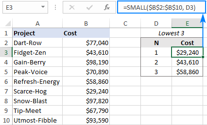
In the table below, suppose you wish to find the bottom 3 values. For this, type the numbers 1, 2 and 3 in separate cells (D3, D4 and D5 in our case). Then, enter the following formula in E3 and drag it down through E5:
=SMALL($B$2:$B$10, D3)
In E3, the formula extracts the smallest value using the number in D3 for the k argument. The key thing is to supply proper cell references due to which the formula copies correctly in other cells: absolute for array and relative for k.
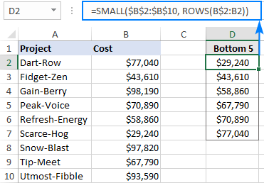
Do not want to bother typing the ranks manually? Use the ROWS function with an expanding range reference to provide the k value. For this, we make an absolute reference for the first cell (or only lock the row coordinate like B$2) and relative reference for the last cell:
=SMALL($B$2:$B$10, ROWS(B$2:B2))
As the result, the range reference expands as the formula is copied down the column. In D2, ROWS(B$2:B2) produces 1 for k, and the formula returns the lowest cost. In D3, ROWS(B$2:B3) yields 2, and we get the 2nd lowest cost, and so on.
Just copy the formula through 5 cells, and you'll get bottom 5 values:
Sum bottom N values
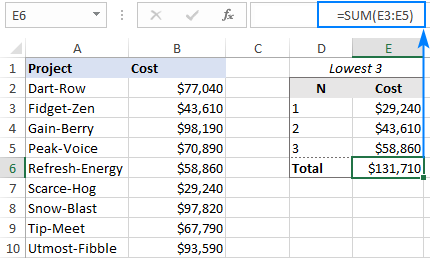
Want to find a total of the smallest n values in a dataset? If you've already extracted the values like shown in the previous example, the easiest solution would be a SUM formula like:
=SUM(E3:E5)
Or you can make an independent formula by using the SMALL function together with SUMPRODUCT:
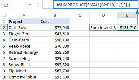
To get the sum of the bottom 3 values in our set of data, the formula takes this shape:
=SUMPRODUCT(SMALL(B2:B10, {1,2,3}))
The SUM function will produce the same result:
=SUM(SMALL(B2:B10, {1,2,3}))
Note. If you use cell references rather than array constant for k, you need to press Ctrl + Shift + Enter to make it an array formula. In Excel 365 that supports dynamic arrays, SUM SMALL works as a regular formula in either case.
How this formula works:
In a regular formula, SMALL returns a single k-th smallest value in a range. In this case, we supply an array constant like {1,2,3} for the k argument, forcing it to return an array of the smallest 3 values:
{29240, 43610, 58860}
The SUMPRODUCT or SUM function adds up the numbers in the array and outputs the total. That's it!
INDEX MATCH SMALL formula to get smallest matches
In situation when you wish to retrieve some data associated with the smallest value, use the classic INDEX MATCH combination with SMALL for the lookup value:
Where:
- Return_array is a range from which to extract associated data.
- Lookup_array is a range where to search for the lowest n-th value.
- N is the position of the smallest value of interest.
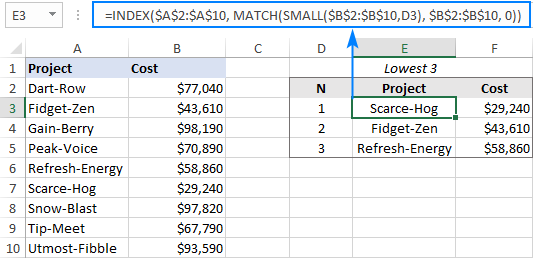
For example, to get the name of the project that has the lowest cost, the formula in E3 is:
=INDEX($A$2:$A$10, MATCH(SMALL($B$2:$B$10, D3), $B$2:$B$10, 0))
Where A2:A10 are the project names, B2:B10 are the costs and D3 is the rank from smallest.
Copy the formula to the below cells (E4 and E5), and you will get the names of the 3 cheapest projects:
Notes:
- This solution works fine for a dataset that has no duplicates. However, two or more duplicate values in a numeric column may create "ties" in ranking, which will lead to wrong results. In this case, please use a bit more sophisticated formula to break ties.
- In Excel 365, this task can be accomplished with the help of the new dynamic array functions. Apart from being much simpler, this approach automatically solves the problem of ties. For full details, please see How to filter bottom N values in Excel.
Sort numbers from lowest to highest with a formula
I believe everyone knows how to put numbers in order with Excel Sort feature. But do you know how to perform sorting with a formula? The users of Excel 365 can do it an easy way with the new SORT function. In Excel 2019, 2016 and earlier versions, SORT does not work, alas. But have a little faith, and SMALL will come to the rescue :)
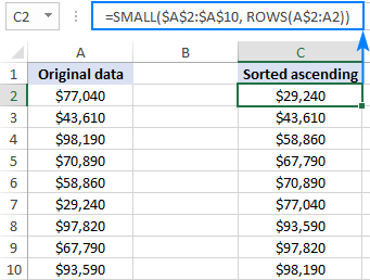
Like in the first example, we use the ROWS function with an expanding range reference to increment k by 1 in every row where the formula is copied:
=SMALL($A$2:$A$10, ROWS(A$2:A2))
Enter the formula in the first cell, and then drag it down to as many cells as there are values in the original data set (C2:C10 in this example):
Tip. To sort descending, use the LARGE function instead of SMALL.
Excel SMALL formula for dates and times
Because dates and times are also numeric values (in the internal Excel system, dates are stored as sequential numbers and times as decimal fractions), the SMALL function can handle them as well without any extra effort on your side.
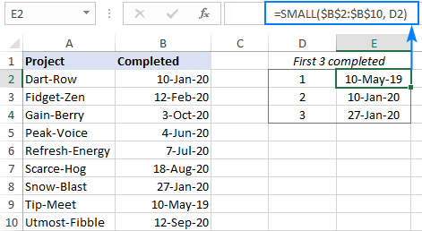
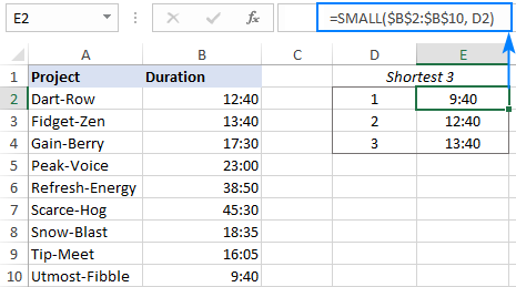
As you can see in the screenshots below, a basic formula that we used for numbers works beautifully for dates and times as well:
=SMALL($B$2:$B$10, D2)
SMALL formula to find the earliest 3 dates:
SMALL formula to get the shortest 3 times:
The next example shows how the SMALL function can help you accomplish a more specific task relating to dates.
Find a previous date closest to today or specified date
In a list of dates, supposing you want to find the nearest date before a specified date. This can be done by using the SMALL function in combination with COUNTIF.
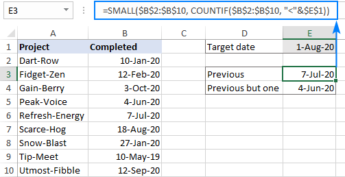
With the list of dates in B2:B10 and the target date in E1, the following formula will return a prior date closest to the target date:
=SMALL(B2:B10, COUNTIF(B2:B10, "<"&E1))
To extract a date that is two dates before the date in E1, i.e. a previous but one date, the formula is:
=SMALL(B2:B10, COUNTIF(B2:B10, "<"&E1)-1)
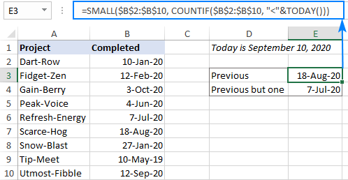
To find a past date closest to today, use the TODAY function for COUNTIF's criteria:
=SMALL(B2:B10, COUNTIF(B2:B10, "<"&TODAY()))
Tip. To prevent errors in situation when a date matching your criteria is not found, you can wrap the IFERROR function around your formula, like this:
=IFERROR(SMALL(B2:B10, COUNTIF(B2:B10, "<"&E1)-1), "Not Found")
How these formulas work:
The general idea is to count the number of dates smaller than the target date with COUNTIF. And this count is exactly what the SMALL function needs for the k argument.
To better grasp the concept, let's look at it from another angle:
If 1-Aug-2020 (the target date in E1) appeared in our dataset, it would be the 7th biggest date on the list. Consequently, there are six dates smaller than it. Meaning, the 6th smallest date is the previous date closest the target date.
So, first we calculate how many dates are smaller than the date in E1 (the result is 6):
COUNTIF(B2:B10, "<"&E1)
And then, plug the count into the 2nd argument of SMALL:
=SMALL(B2:B10, 6)
To get the previous but one date (which is the 5th smallest date in our case), we subtract 1 from COUNTIF's result.
How to highlight bottom values in Excel
To highlight the smallest n values in your table with Excel conditional formatting, you can use either a built-in Top/Bottom option or set up your own rule based on a SMALL formula. The first method is faster and easier to apply, while the second provides more control and flexibility. The below steps will walk you through creating a custom rule:
- Select the range in which you want to highlight bottom values. In our case, the numbers are in B2:B10, so we select it. If you'd like to highlight entire rows, then select A2:B10.
- On the Home tab, in the Styles group, click Conditional formatting > New Rule.
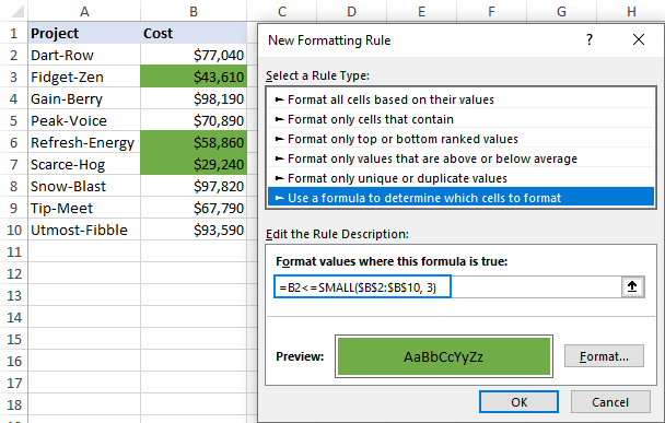
- In the New Formatting Rule dialog box, choose Use a formula to determine which cells to format.
- In the Format values where this formula is true box, enter a formula like this one:
=B2<=SMALL($B$2:$B$10, 3)Where B2 is the leftmost cell of the numeric range to be checked, $B$2:$B$10 is the whole range, and 3 is the n bottom values to highlight.
In your formula, please mind the reference types: the leftmost cell is a relative reference (B2) while the range is the absolute reference ($B$2:$B$10).
- Click the Format button and choose any format you like.
- Click OK twice to close both dialog windows.
Done! The bottom 3 values in column B are highlighted:
For more information, please see Excel conditional formatting based on formula.
Excel SMALL function not working
As you've just seen from our examples, using the SMALL function in Excel is quite easy, and you are unlikely to have any difficulties with it. If your formula does not work, most likely that will be a #NUM! error, which may occur because of the following reasons:
- Array is empty or does not contain a single numeric value.
- The k value is less than zero (a silly typo can cost you hours of troubleshooting!) or exceeds the number of values in the array.
That's how to use a SMALL formula in Excel to find and highlight bottom numbers in a set of data. If you know any other scenarios where the function comes in handy, you are most welcome to share in comments. I thank you for reading and hope to see you on our blog next week!
Practice workbook for download
Excel SMALL formula examples (.xlsx file)
 by
by
One comment
How do I use the SMALL function for picking out the 10 lowest numbers of 20 numbers