The tutorial explains how to add and where to find Solver in different Excel versions, from 2016 to 2003. Step-by-step examples show how to use Excel Solver to find optimal solutions for linear programming and other kinds of problems.
Everyone knows that Microsoft Excel contains a lot of useful functions and powerful tools that can save you hours of calculations. But did you know that it also has a tool that can help you find optimal solutions for decision problems?
In this tutorial, we are going to cover all essential aspects of the Excel Solver add-in and provide a step-by-step guide on how to use it most effectively.
What is Excel Solver?
Excel Solver belongs to a special set of commands often referred to as What-if Analysis Tools. It is primarily purposed for simulation and optimization of various business and engineering models.
The Excel Solver add-in is especially useful for solving linear programming problems, aka linear optimization problems, and therefore is sometimes called a linear programming solver. Apart from that, it can handle smooth nonlinear and non-smooth problems. Please see Excel Solver algorithms for more details.
While Solver can't crack every possible problem, it is really helpful when dealing with all kinds of optimization problems where you need to make the best decision. For example, it can help you maximize the return of investment, choose the optimal budget for your advertising campaign, make the best work schedule for your employees, minimize the delivery costs, and so on.
How to add Solver to Excel
The Solver add-in is included with all versions of Microsoft Excel beginning with 2003, but it is not enabled by default.
To add Solver to your Excel, perform the following steps:
- In Excel 2010 - Excel 365, click File > Options.
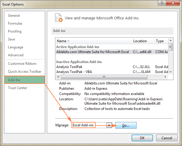
In Excel 2007, click the Microsoft Office button, and then click Excel Options. - In the Excel Options dialog, click Add-Ins on the left sidebar, make sure Excel Add-ins is selected in the Manage box at the bottom of the window, and click Go.
- In the Add-Ins dialog box, check the Solver Add-in box, and click OK:
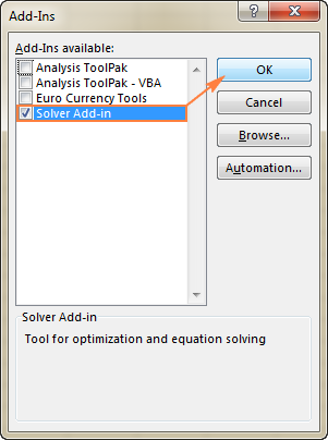
To get Solver on Excel 2003, go to the Tools menu, and click Add-Ins. In the Add-Ins available list, check the Solver Add-in box, and click OK.
Note. If Excel displays a message that the Solver Add-in is not currently installed on your computer, click Yes to install it.
Where is Solver in Excel?
In the modern versions of Excel, the Solver button appears on the Data tab, in the Analysis group:

Where is Solver in Excel 2003?
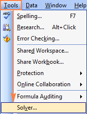
After the Solver Add-in is loaded to Excel 2003, its command is added to the Tools menu:
Now that you know where to find Solver in Excel, open a new worksheet and let's get started!
Note. The examples discussed in this tutorial use Solver in Excel 2013. If you have another Excel version, the screenshots may not match your version exactly, although the Solver functionality is basically the same.
How to use Solver in Excel
Before running the Excel Solver add-in, formulate the model you want to solve in a worksheet. In this example, let's find a solution for the following simple optimization problem.
Problem. Supposing, you are the owner of a beauty salon and you are planning on providing a new service to your clients. For this, you need to buy a new equipment that costs $40,000, which should be paid by instalments within 12 months.
Goal: Calculate the minimal cost per service that will let you pay for the new equipment within the specified timeframe.
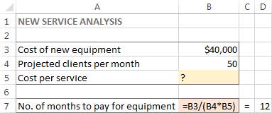
For this task, I've created the following model:
And now, let's see how Excel Solver can find a solution for this problem.
1. Run Excel Solver
On the Data tab, in the Analysis group, click the Solver button.
2. Define the problem
The Solver Parameters window will open where you have to set up the 3 primary components:
- Objective cell
- Variable cells
- Constraints
Exactly what does Excel Solver do with the above parameters? It finds the optimal value (maximum, minimum or specified) for the formula in the Objective cell by changing the values in the Variable cells, and subject to limitations in the Constraints cells.
Objective
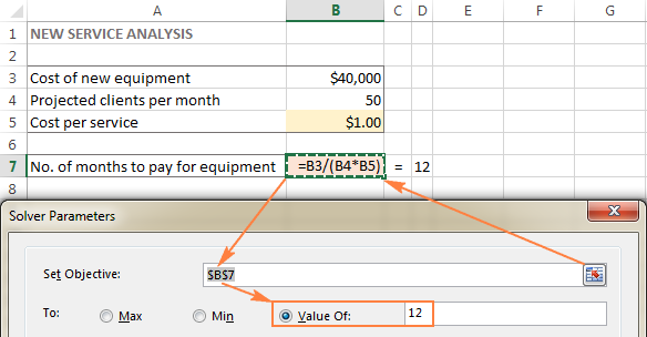
The Objective cell (Target cell in earlier Excel versions) is the cell containing a formula that represents the objective, or goal, of the problem. The objective can be to maximize, minimize, or achieve some target value.
In this example, the objective cell is B7, which calculates the payment term using the formula =B3/(B4*B5) and the result of the formula should be equal to 12:
Variable cells
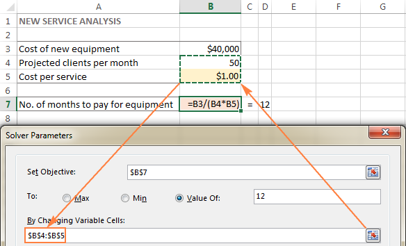
Variable cells (Changing cells or Adjustable cells in earlier versions) are cells that contain variable data that can be changed to achieve the objective. Excel Solver allows specifying up to 200 variable cells.
In this example, we have a couple of cells whose values can be changed:
- Projected clients per month (B4) that should be less than or equal to 50; and
- Cost per service (B5) that we want Excel Solver to calculate.
Tip. If the variable cells or ranges in your model are non-adjacent, select the first cell or range, and then press and hold the Ctrl key while selecting other cells and/or ranges. Or, type the ranges manually, separated with commas.
Constraints
The Excel Solver Constrains are restrictions or limits of the possible solutions to the problem. To put it differently, constraints are the conditions that must be met.
To add a constraint(s), do the following:
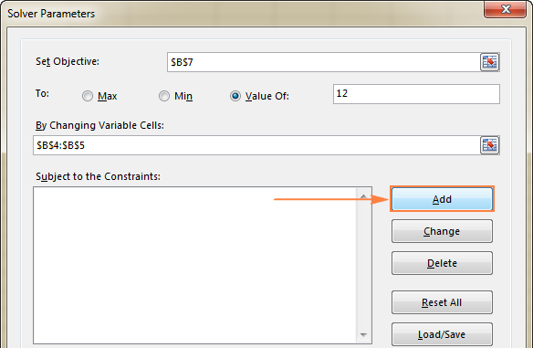
- Click the Add button right to the "Subject to the Constraints" box.
- In the Constraint window, enter a constraint.
- Click the Add button to add the constraint to the list.

- Continue entering other constraints.
- After you have entered the final constraint, click OK to return to the main Solver Parameters window.
Excel Solver allows specifying the following relationships between the referenced cell and the constraint.
- Less than or equal to, equal to, and greater than or equal to. You set these relationships by selecting a cell in the Cell Reference box, choosing one of the following signs: <=, =, or >=, and then typing a number, cell reference / cell name, or formula in the Constraint box (please see the above screenshot).
- Integer. If the referenced cell must be an integer, select int, and the word integer will appear in the Constraint box.
- Different values. If each cell in the referenced range must contain a different value, select dif, and the word AllDifferent will appear in the Constraint box.
- Binary. If you want to limit a referenced cell either to 0 or 1, select bin, and the word binary will appear in the Constraint box.
Note. The int, bin, and dif relationships can only be used for constraints on Variable cells.
To edit or delete an existing constraint do the following:
- In the Solver Parameters dialog box, click the constraint.
- To modify the selected constraint, click Change and make the changes you want.
- To delete the constraint, click the Delete button.
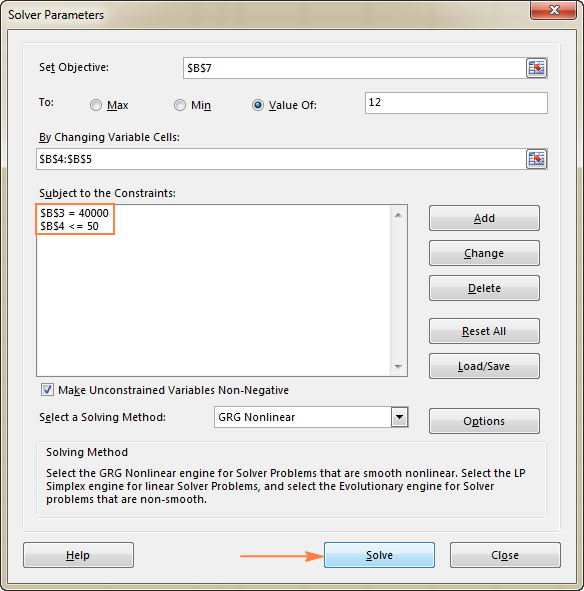
In this example, the constraints are:
- B3=40000 - cost of the new equipment is $40,000.
- B4<=50 - the number of projected patients per month in under 50.
3. Solve the problem
After you've configured all the parameters, click the Solve button at the bottom of the Solver Parameters window (see the screenshot above) and let the Excel Solver add-in find the optimal solution for your problem.
Depending on the model complexity, computer memory and processor speed, it may take a few seconds, a few minutes, or even a few hours.
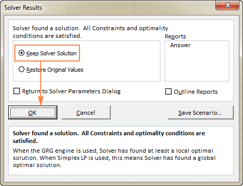
When Solver has finished processing, it will display the Solver Results dialog window, where you select Keep the Solver Solution and click OK:
The Solver Result window will close and the solution will appear on the worksheet right away.
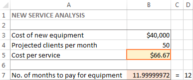
In this example, $66.67 appears in cell B5, which is the minimal cost per service that will let you pay for the new equipment in 12 months, provided there are at least 50 clients per month:
Tips:
- If the Excel Solver has been processing a certain problem for too long, you can interrupt the process by pressing the Esc key. Excel will recalculate the worksheet with the last values found for the Variable cells.
- To get more details about the solved problem, click a report type in the Reports box, and then click OK. The report will be created on a new worksheet:

Now that you've got the basic idea of how to use Solver in Excel, let's have a closer look at a couple more examples that might help you gain more understanding.
Excel Solver examples
Below you will find two more examples of using the Excel Solver addin. First, we will find a solution for a well-known puzzle, and then solve a real-life linear programming problem.
Excel Solver example 1 (magic square)
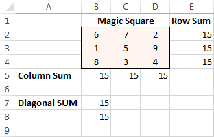
I believe everyone is familiar with "magic square" puzzles where you have to put a set of numbers in a square so that all rows, columns and diagonals add up to a certain number.
For instance, do you know a solution for the 3x3 square containing numbers from 1 to 9 where each row, column and diagonal adds up to 15?
It's probably no big deal to solve this puzzle by trial and error, but I bet the Solver will find the solution faster. Our part of the job is to properly define the problem.
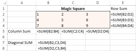
To begin with, enter the numbers from 1 to 9 in a table consisting of 3 rows and 3 columns. The Excel Solver does not actually need those numbers, but they will help us visualize the problem. What the Excel Solver add-in really needs are the SUM formulas that total each row, column and 2 diagonals:
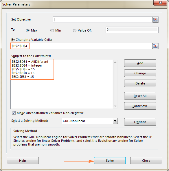
With all the formulas in place, run Solver and set up the following parameters:
- Set Objective. In this example, we don't need to set any objective, so leave this box empty.
- Variable Cells. We want to populate numbers in cells B2 to D4, so select the range B2:D4.
- Constraints. The following conditions should be met:
- $B$2:$D$4 = AllDifferent - all of the Variable cells should contain different values.
- $B$2:$D$4 = integer - all of the Variable cells should be integers.
- $B$5:$D$5 = 15 - the sum of values in each column should equal 15.
- $E$2:$E$4 = 15 - the sum of values in each row should equal 15.
- $B$7:$B$8 = 15 - the sum of both diagonals should equal 15.
Finally, click the Solve button, and the solution is there!
Excel Solver example 2 (linear programming problem)
This is an example of a simple transportation optimization problem with a linear objective. More complex optimization models of this kind are used by many companies to save thousands of dollars each year.
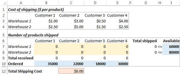
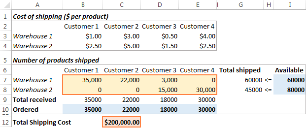
Problem: You want to minimize the cost of shipping goods from 2 different warehouses to 4 different customers. Each warehouse has a limited supply and each customer has a certain demand.
Goal: Minimize the total shipping cost, not exceeding the quantity available at each warehouse, and meeting the demand of each customer.
Source data
Here is how our transportation optimization problem looks like:
Formulating the model
To define our linear programming problem for the Excel Solver, let's answer the 3 main questions:
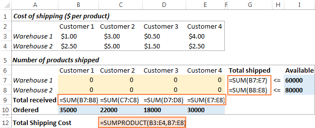
- What decisions are to be made? We want to calculate the optimal quantity of goods to deliver to each customer from each warehouse. These are Variable cells (B7:E8).
- What are the constraints? The supplies available at each warehouse (I7:I8) cannot be exceeded, and the quantity ordered by each customer (B10:E10) should be delivered. These are Constrained cells.
- What is the goal? The minimal total cost of shipping. And this is our Objective cell (C12).
The next thing for you to do is to calculate the total quantity shipped from each warehouse (G7:G8), and the total goods received by each customer (B9:E9). You can do this with simple Sum formulas demonstrated in the below screenshot. Also, insert the SUMPRODUCT formula in C12 to calculate the total cost of shipping:
To make our transportation optimization model easier to understand, create the following named ranges:
| Range name | Cells | Solver parameter |
| Products_shipped | B7:E8 | Variable cells |
| Available | I7:I8 | Constraint |
| Total_shipped | G7:G8 | Constraint |
| Ordered | B10:E10 | Constraint |
| Total_received | B9:E9 | Constraint |
| Shipping_cost | C12 | Objective |
The last thing left for you to do is configure the Excel Solver parameters:
- Objective: Shipping_cost set to Min
- Variable cells: Products_shipped
- Constraints: Total_received = Ordered and Total_shipped <= Available
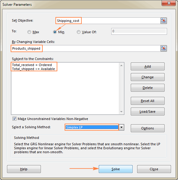
Please pay attention that we've chosen the Simplex LP solving method in this example because we are dealing with the linear programming problem. If you are not sure what kind of problem yours is, you can leave the default GRG Nonlinear solving method. For more information, please see Excel Solver algorithms.
Solution
Click the Solve button at the bottom of the Solver Parameters window, and you will get your answer. In this example, the Excel Solver add-in calculated the optimal quantity of goods to deliver to each customer from each warehouse with the minimal total cost of shipping:
And here is one more example of practical use: Find all combinations that equal given sum with Excel Solver.
How to save and load Excel Solver scenarios
When solving a certain model, you may want to save your Variable cell values as a scenario that you can view or re-use later.
For example, when calculating the minimal service cost in the very first example discussed in this tutorial, you may want to try different numbers of projected clients per month and see how that affects the service cost. At that, you may want to save the most probable scenario you've already calculated and restore it at any moment.
Saving an Excel Solver scenario boils down to selecting a range of cells to save the data in. Loading a Solver model is just a matter of providing Excel with the range of cells where your model is saved. The detailed steps follow below.
Saving the model
To save the Excel Solver scenario, perform the following steps:
- Open the worksheet with the calculated model and run the Excel Solver.
- In the Solver Parameters window, click the Load/Save button.

- Excel Solver will tell you how many cells are needed to save your scenario. Select that many empty cells and click Save:
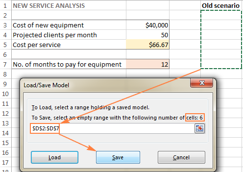
- Excel will save your current model, which may look something similar to this:

At the same time, the Solver Parameters window will show up where you can change your constraints and try different "what if" options.
Loading the saved model
When you decide to restore the saved scenario, do the following:
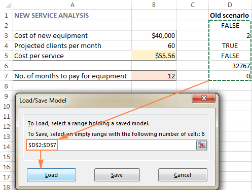
- In the Solver Parameters window, click the Load/Save button.
- On the worksheet, select the range of cells holding the saved model and click Load:
- In the Load Model dialog, click the Replace button:
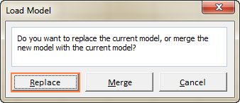
- This will open the main Excel Solver window with the parameters of the previously saved model. All you need to do is to click the Solve button to re-calculate it.
Excel Solver algorithms
When defining a problem for the Excel Solver, you can choose one of the following methods in the Select a Solving Method dropdown box:
To change how Solver finds a solution, click the Options button in the Solver Parameters dialog box, and configure any or all options on the GRG Nonlinear, All Methods, and Evolutionary tabs.
This is how you can use Solver in Excel to find the best solutions for your decision problems. At the end of this post, you can download the sample workbook with all the examples discussed in this tutorial and reverse-engineer them for better understanding. I thank you for reading and hope to see you on our blog next week.
Practice workbook for download
Excel Solver examples (.xlsx file)
 by
by
6 comments
In the example in "How to use Solver in Excel", why do you define a constraint for B2, when it is not one of the variable cells? I have tried deleting that constraint and the solution is the same.
In the analysis of the solution you say "provided there are at least 50 clients per month" when the condition B4<=50 means that you have "at most 50 clients per month".
Otherwise, nice instructions. Very helpful.
Hi Oscar,
Thank you for your questions.
We define a constraint for B3 because it contains a condition that should be met (cost of the new equipment is $40,000 - it's a fixed amount). Variable cells are B4 and B5.
The phrase "provided there are at least 50 clients per month" relates to a particular solution shown in the screenshot - cost per service ($66.67) was calculated assuming there are 50 clients per month (see the value in B4). B4<=50 was the condition for Solver.
I tried the Magic Square one with my students and we were not able to solve it as directed. We received error messages, such as "An AllDifferent Constraint must have either no bounds, or a lower bound of 1 and and upper bound of N, where N is the number of cells in the Constraint." However, we could not figure out where to set this parameter.
Can anyone help with this?
Hi Michelle,
To figure out the source of the problem, you can download our sample workbook and compare our Magic Square model with yours.
hello,
please i was giving this assignment but i am finding it hard to understand it. please can any one help me solve it?
To create a Linear Programming model using MS Excel Solver (25%)
A metal works manufacturing company produces four products fabricated from sheet metal in a
production line that consist of four operations: 1) Stamping, 2) Assembly, 3) Finishing and 4)
Packaging. The processing times per unit for each operation and total available hours per month
are as follows:
Product (hour/unit)
Operation 1 2 3 4 Total Hours available per
month
Stamping 0.07 0.2 0.1 0.15 700
Assembly 0.15 0.18 -- 0.12 450
Finishing 0.08 0.21 0.06 0.10 600
Packaging 0.12 0.15 0.08 0.12 500
5
The sheet metal required for each product, the maximum demand per month, the minimum
required contracted production, and the profit per product are given as follows:
Monthly sales demand
Product Sheet Metal (ft2
) Minimum Maximum Profit(£)
1 2.1 300 3,000 9
2 1.5 200 1,400 10
3 2.8 400 4,200 8
4 3.1 300 1,800 12
The company has 5,200 square feet of fabricated metal available each month.
Formulate a linear programming model and use Excel Solver function to suggest the best mix of
products which would result in the highest profit within the given constraints.
Can u better rephrase or construct the question properly