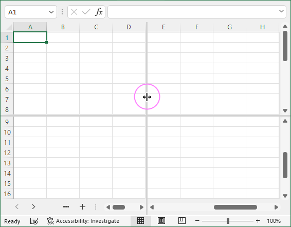
In this article, you'll learn how to display certain rows and/or columns in separate panes by splitting the worksheet into two or four parts.
When working with large datasets, it can be helpful to see a few areas of the same worksheet at a time to compare different subsets of data. This can be done by using Excel's Split Screen feature.
How to split screen in Excel
Splitting is a one-click operation in Excel. To split up a worksheet into two or four parts, this is what you need to do:
- Select the row/column/cell before which you want to place the split.
- On the View tab, in the Windows group, click the Split button.
Done!

Depending on your selection, the worksheet window can be divided horizontally, vertically or both, so you have two or four separate sections with their own scrollbars. Let's see how each scenario works.
Split worksheet vertically on columns
To separate two areas of the spreadsheet vertically, select the column to the right of the column where you wish the split to appear and click the Split button.
In the dataset below, suppose you want to display the item details (columns A through C) and sales numbers (columns D through H) in separate panes. To have it done, select column D on the left of which the split should be made:

As the result, the worksheet is divided into two vertical panes, each having its own scrollbar.

Now that the first three columns are locked by the split, you can select any cell in the right-hand pane and scroll to the right. This will hide columns D through F from view, focusing your attention on the more important column G:

Split worksheet horizontally on rows
To separate your Excel window horizontally, select the row below the row where you want the split to occur.
Let's say you aim to compare data for East and West regions. As the West data begin in row 10, we have it selected:

The window gets divided into two panes, one above the other. And now, you can bring any part of each pane to focus by using two vertical scrollbars.

Split worksheet into four parts
To view four different sections of the same worksheet simultaneously, split your screen both vertically and horizontally. For this, select the cell above and to the left of which the split should appear, and then use the Split command.
In the image below, cell G10 is selected, so the screen is separated into the following parts:

Working with split bars
By default, the split always occurs above and to the left of the active cell.
If cell A1 is selected, the worksheet will be divided into four equal parts.

If a wrong cell was accidentally selected, you can adjust the panes by dragging the split bar to the desired position using the mouse.

How to remove split
To undo the worksheet splitting, just click the Split button again. Another easy way is to double click the split bar.
How to split screen between two worksheets
The Excel Split feature only works within a single spreadsheet. To view two tabs in the same workbook at a time, you need to open another window of the same workbook as explained in View two Excel sheets side by side.
That's how the Excel Split Screen feature works. Hope you find our tips helpful. If there's something else you'd like us to share next time, please let us know in comments. I thank you for reading and look forward to seeing you on our blog next week!
 by
by