The tutorial explains how to do sum in Excel by using the AutoSum feature, and how to make your own SUM formula to total a column, row or selected range. You will also learn how to sum only visible cells, calculate running total, sum across sheets, and find out why your Excel Sum formula is not working.
If you want a quick sum of certain cells in Excel, you can simply select those cells, and look at the status bar at the bottom right corner of your Excel window:

For something more permanent, use the Excel SUM function. It is very simple and straightforward, so even if you are a beginner in Excel, you will hardly have any difficulty in understanding the following examples.
How to sum in Excel using a simple arithmetic calculation
If you need a quick total of several cells, you can use Microsoft Excel as a mini calculator. Just utilize the plus sign operator (+) like in a normal arithmetic operation of addition. For example:
=1+2+3
or
=A1+C1+D1

However, if you need to sum a few dozen or a few hundred rows, referencing each cell in a formula does not sound like a good idea. In this case, you can use the Excel SUM function specially designed to add a specified set of numbers.
How to use SUM function in Excel
Excel SUM is a math and trig function that adds values. The syntax of the SUM function is as follows:
The first argument is required, other numbers are optional, and you can supply up to 255 numbers in a single formula.
In your Excel SUM formula, each argument can be a positive or negative numeric value, range, or cell reference. For example:
=SUM(A1:A100)
=SUM(A1, A2, A5)
=SUM(1,5,-2)
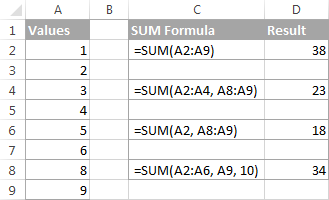
The Excel SUM function is useful when you need to add up values from different ranges, or combine numeric values, cell references and ranges. For example:
=SUM(A2:A4, A8:A9)
=SUM(A2:A6, A9, 10)
The below screenshot shows these and a few more SUM formula examples:
In real-life worksheets, the Excel SUM function is often included in bigger formulas as part of more complex calculations.
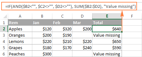
For example, you can embed SUM in the value_if_true argument of the IF function to add numbers in columns B, C and D if all three cells in the same row contain values, and show a warning message if any of the cells is blank:
=IF(AND($B2<"", $C2<>"", $D2<>""), SUM($B2:$D2), "Value missing")
And here's another example of using an advanced SUM formula in Excel: VLOOKUP and SUM formula to total all matching values.
How to AutoSum in Excel
If you need to sum one range of numbers, whether a column, row or several adjacent columns or rows, you can let Microsoft Excel write an appropriate SUM formula for you.
Simply select a cell next to the numbers you want to add, click AutoSum on the Home tab, in the Editing group, press the Enter key, and you will have a Sum formula inserted automatically:
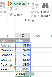
As you can see in the following screenshot, Excel's AutoSum feature not only enters a Sum formula, but also selects the most likely range of cells that you'd want to total. Nine times out of ten, Excel gets the range right. If not, you can manually correct the range by simply dragging the cursor through the cells to sum, and then hit the Enter key.
Tip. A faster way to do AutoSum in Excel is to use the Sum shortcut Alt + =. Just hold the Alt key, press the Equal Sign key, and then hit Enter to complete an automatically inserted Sum formula.
Apart from calculating total, you can use AutoSum to automatically enter AVERAGE, COUNT, MAX, or MIN functions. For more information, please check out the Excel AutoSum tutorial.
How to sum a column in Excel
To sum numbers in a specific column, you can use either the Excel SUM function or AutoSum feature.
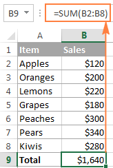
For example, to sum values in column B, say in cells B2 to B8, enter the following Excel SUM formula:
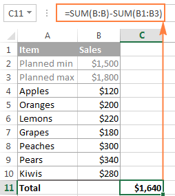
If a column you want to sum has a variable number of rows (i.e. new cells can be added and existing ones can be deleted at any time), you can sum the entire column by supplying a column reference, without specifying a lower or upper bound. For example: Important note! In no case you should put your 'Sum of a column' formula in the column you want to total because this would create a circular cell reference (i.e. an endless recursive summation), and your Sum formula would return 0. Usually, supplying a column reference to the Excel Sum formula totals the entire column ignoring the header, as demonstrated in the above screenshot. But in some cases, the header of the column you want to total can actually have a number in it. Or, you may want to exclude the first few rows with numbers that are not relevant to the data you want to sum. Regrettably, Microsoft Excel does not accept a mixed SUM formula with an explicit lower bound but without an upper bound like =SUM(B2:B), which works fine in Google Sheets. To exclude the first few rows from summation, you can use one of the following workarounds. For example, to sum column B without the header (i.e. excluding cell B1), you can use the following formulas:=SUM(B2:B8)
Total an entire column with indefinite number of rows
=SUM(B:B)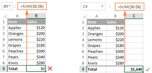
Sum column except header or excluding a few first rows
=SUM(B:B)-SUM(B1:B3)
=SUM(B2:B1048576)
=SUM(B2:B655366)
How to sum rows in Excel
Similarly to totaling a column, you can sum a row in Excel by using the SUM function, or have AutoSum to insert the formula for you.
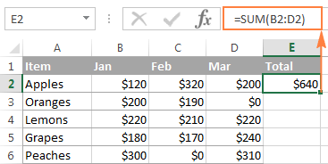
For example, to add values in cells B2 to D2, use the following formula:
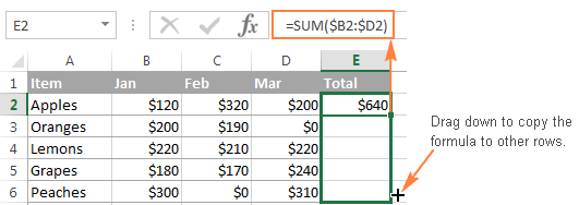
To add values in each row individually, just drag down your Sum formula. The key point is to use relative (without $) or mixed cell references (where the $ sign fixes only the columns). For example: To total the values in a range containing several rows, simply specify the desired range in the Sum formula. For example: To sum the entire row with an indefinite number of columns, supply a whole-row reference to your Excel Sum formula, e.g.: Please remember that you shouldn't enter that 'Sum of a row' formula in any cell of the same row to avoid creating a circular reference because this would result in a wrong calculation, if any:
To sum rows excluding a certain column(s), total the entire row and then subtract irrelevant columns. For example, to sum row 2 except the first 2 columns, use the following formula:=SUM(B2:D2)
How to sum multiple rows in Excel
=SUM($B2:$D2)
=SUM(B2:D6) - sums values in rows 2 to 6.=SUM(B2:D3, B5:D6) - sums values in rows 2, 3, 5 and 6.
How to sum a whole row
=SUM(2:2)
=SUM(2:2)-SUM(A2:B2)
Use Excel Total Row to sum data in a table
If your data is organized in an Excel table, you can benefit from the special Total Row feature that can quickly sum the data in your table and display totals in the last row.
A big advantage of using Excel tables is that they auto-expand to include new rows, so any new data you input in a table will be included in your formulas automatically. If can learn about other benefits of Excel tables in this article: 10 most useful features of Excel tables.
To convert an ordinary range of cells into a table, select it and press Ctrl + T shortcut (or click Table on the Insert tab).
How to add a total row in Excel tables
Once your data is arranged in a table, you can insert a total row in this way:
- Click anywhere in the table to display the Table Tools with the Design tab.
- On the Design tab, in the Table Style Options group, select the Total Row box:

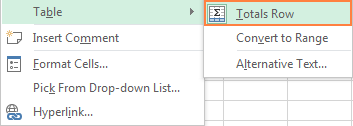
Another way to add a total row in Excel is to right click any cell within the table, and then click Table > Totals Row.
How to total data in your table
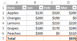
When the total row appears at the end of the table, Excel does its best to determine how you would like to calculate data in the table.
In my sample table, the values in column D (rightmost column) are added automatically and the sum is displayed in the Total Row:
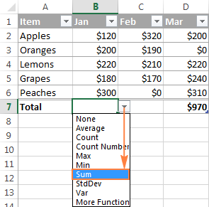
To total values in other columns, simply select a corresponding cell in the total row, click the drop-down list arrow, and select Sum:
If you want to perform some other calculation, select the corresponding function from the drop-down list such as Average, Count, Max, Min, etc.
If the total row automatically displays a total for a column that doesn't need one, open the dropdown list for that column and select None.
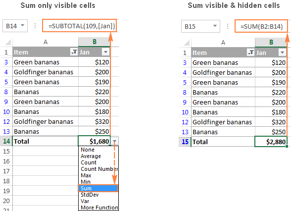
Note. When using the Excel Total Row feature to sum a column, Excel totals values only in visible rows by inserting the SUBTOTAL function with the first argument set to 109. You will find the detailed explanation of this function in the next section.
If you want to sum data both in visible and invisible rows, do not add the total row, and use a normal SUM function instead:
How to sum only filtered (visible) cells in Excel
Sometimes, for more effective date analysis, you may need to filter or hide some data in your worksheet. A usual Sum formula won't work in this case because the Excel SUM function adds all values in the specified range including the hidden (filtered out) rows.
If you want to sum only visible cells in a filtered list, the fastest way is to organize your data in an Excel table, and then turn on the Excel Total Row feature. As demonstrated in the previous example, selecting Sum in a table's total row inserts the SUBTOTAL function that ignores hidden cells.
Another way to sum filtered cells in Excel is to apply an AutoFilter to your data manually by clicking the Filter button on the Data tab. And then, write a Subtotal formula yourself.
The SUBTOTAL function has the following syntax:
Where:
- Function_num- a number from 1 to 11 or from 101 to 111 that specifies which function to use for the subtotal.
You can find the full list of functions on support.office.com. For now, we are interested only in the SUM function, which is defined by numbers 9 and 109. Both numbers exclude filtered-out rows. The difference is that 9 includes cells hidden manually (i.e. right-click > Hide), while 109 excludes them.
So, if you are looking to sum only visible cells, regardless of how exactly irrelevant rows were hidden, then use 109 in the first argument of your Subtotal formula.
- Ref1, Ref2, … - cells or ranges that you want to subtotal. The first Ref argument is required, others (up to 254) are optional.
In this example, let's sum visible cells in range B2:B14 by using the following formula:
=SUBTOTAL(109, B2:B14)
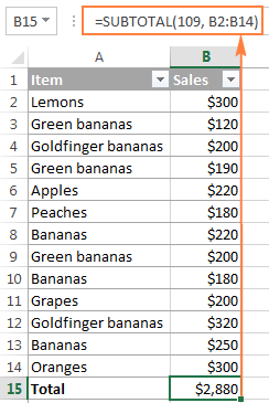
And now, let's filter only 'Banana' rows and make sure that our Subtotal formula sums only visible cells:
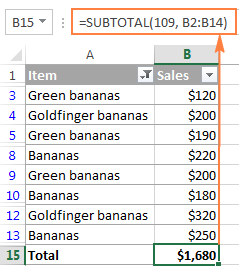
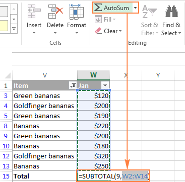
Tip. You can have Excel's AutoSum feature to insert the Subtotal formula for you automatically. Just organize your data in table (Ctrl + T) or filter the data the way you want by clicking the Filter button. After that, select the cell immediately below the column you want to total, and click the AutoSum button on the ribbon. A SUBTOTAL formula will be inserted, summing only the visible cells in the column.
How to do a running total (cumulative sum) in Excel
To calculate a running total in Excel, you write a usual SUM formula with a clever use of absolute and relative cells references.
For example, to display the cumulative sum of numbers in column B, enter the following formula in C2, and then copy it down to other cells:
=SUM($B$2:B2)
The relative reference B2 will change automatically based on the relative position of the row in which the formula is copied:
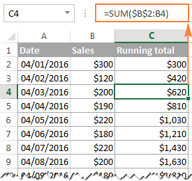
You can find the detailed explanation of this basic Cumulative Sum formula and tips on how to improve it in this tutorial: How to calculate running total in Excel.
How to sum across sheets
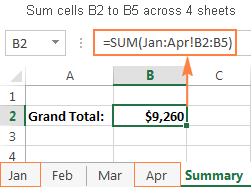
If you have several worksheets with the same layout and the same data type, you can add the values in the same cell or in the same range of cells in different sheets with a single SUM formula.
A so-called 3-D reference is what does the trick:
=SUM(Jan:Apr!B6)
Or
=SUM(Jan:Apr!B2:B5)
The first formula adds values in cell B6, while the second formula sums the range B2:B5 in all worksheets located between the two boundary sheets that you specify (Jan and Apr in this example):
You can find more information about a 3-d reference and the detailed steps to create such formulas in this tutorial: How to create a 3-D reference to calculate multiple sheets.
Excel conditional sum
If your task requires adding only those cells that meet a certain condition or a few conditions, you can use the SUMIF or SUMIFS function, respectively.
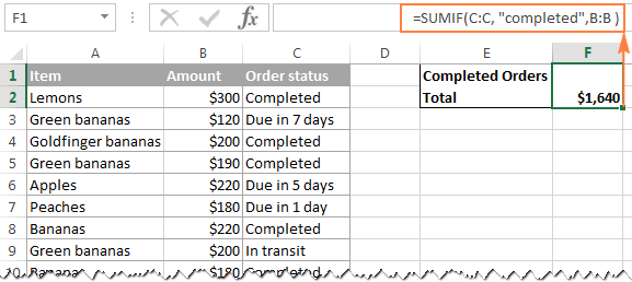
For example, the following SUMIF formula adds only those amounts in column B that have "Completed" status in column C:
=SUMIF(C:C,"completed",B:B )
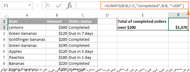
To calculate a conditional sum with multiple criteria, use the SUMIFS function. In the above example, to get the total of "Completed" orders with the amount over $200, use the following SUMIFS formula:
=SUMIFS(B:B,C:C,"completed",B:B, ">200" )
You can find the detailed explanation of the SUMIF and SUMIFS syntax and plenty more formula examples in these tutorials:
- SUMIF function in Excel: examples for numbers, dates, text, blanks and not blanks
- SUMIF in Excel - formula examples to conditionally sum cells
- How to use Excel SUMIFS and SUMIF with multiple criteria
Note. The Conditional Sum functions are available in Excel versions beginning with Excel 2003 (more precisely, SUMIF was introduced in Excel 2003, while SUMIFS only in Excel 2007). If someone still uses an earlier Excel version, you'd need to make an array SUM formula as demonstrated in Using Excel SUM in array formulas to conditionally sum cells.
Excel SUM not working - reasons and solutions
Are you trying to add a few values or total a column in your Excel sheet, but a simple SUM formula doesn't compute? Well, if the Excel SUM function is not working, it's most likely because of the following reasons.
1. #Name error appears instead of the expected result
It's the easiest error to fix. In 99 out of 100 cases, the #Name error indicates that the SUM function is misspelled.
2. Some numbers are not added
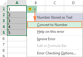
Another common reason for a Sum formula (or Excel AutoSum) not working are numbers formatted as text values. At first sight, they look like normal numbers, but Microsoft Excel perceives them as text strings and leaves them out of calculations.
One of the visual indicators of text-numbers are the default left alignment and green triangles in top-left corner of the cells, like in the right-hand sheet in the below screenshot:

To fix this, select all problematic cells, click the warning sign, and then click Convert to Number.
If against all expectations that does not work, try other solutions described in: How to fix numbers formatted as text.
3. Excel SUM function returns 0
Apart from numbers formatted as text, a circular reference is a common source of problem in Sum formulas, especially when you are trying to total a column in Excel. So, if your numbers are formatted as numbers, but your Excel Sum formula still returns zero, trace and fix the circular references in your sheet (Formula tab > Error Checking > Circular Reference). For the detailed instructions, please see How to find a circular reference in Excel.
4. Excel Sum formula returns a higher number than expected
If against all expectations your Sum formula returns a bigger number than it should, remember that the SUM function in Excel adds both visible and invisible (hidden) cells. In this case, use the Subtotal function instead, as demonstrated in How to sum only visible cells in Excel.
5. Excel SUM formula not updating
When a SUM formula in Excel continues to show the old total even after you've updated the values in the dependent cells, most likely Calculation Mode is set to Manual. To fix this, go to the Formulas tab, click the dropdown arrow next to Calculate Options, and click Automatic.
Well, these are the most common reasons for SUM not working in Excel. If none of the above is your case, check out other possible reasons and solutions: Excel formulas not working, not updating, not calculating.
This is how you use a SUM function in Excel. I thank you for reading and hope to see you on our blog next week!
Practice workbook for download
Excel SUM function - examples (.xlsx file)
 by
by
33 comments
Hello, I need help with correct formula: I have Column A3 cell for part numbers, Column B3 Cell for total inventory qty, Column C3 for W/O, Column D3 total after p/n used then rest of roll similar to C3 and D3 all way to Y3 and Z3. C2 and D2 are merge together as drop list for either W/O open or closed between each two cells. How do you sum qty for every other column if W/O is open and not sum if w/o is closed?
Thank You
I have figure out the formula for this.
=SUMIFS(O3:BA3,O1:BA1,"open")
how to use subtotal formula with multiple criteria when data was filtered?
Hello!
The answer to your question can be found in this article: Excel SUBTOTAL function with formula examples.
i want to set formula in excel which data is below please help me to set formula ....i have attached excel sheet also.
---------------------------------------------------------------------------------
RECV DATE | RCV. CH. NO | RECV | RECV DATE | RCV. CH. NO | RECV |
---------------------------------------------------------------------------------
02-Aug | 1362 | 717 | 02-Aug | 1366 | 612 |
---------------------------------------------------------------------------------
my data is in column wise and i want datewise total sum of "RECV" values ...
please help me
Hi!
To calculate the sum of values by date, use the SUMIF function. See here for detailed instructions and examples.
I cannot get Autosum to return an answer when I sum up cells in the same row. I simply see the formula appear but not the answer.
go to formula bar than click show formula.....
Hi
I use this formula to hide zero =IF(SUM(E7:P7)=0,"",SUM(E7:P7)). In another cell when I want to subtract some value from this zero hide formula cell it results in #value! please give me the formula to get rid of the error value, hope will get it soon. Thanks in advance
Hello!
To avoid calculation problems, do not replace zero with an empty cell or space. Use a custom number format as described in this tutorial: Display zeroes as dashes or blanks. I hope my advice will help you solve your task.
I want to be able to find the top 10 results in a row list. I have the names in column A, then after each competition i have a column with the score and then points awarded. I have 15 competitions each with a score and points. I want to total the best 10 results for each person from the total of the points and exclude the score. I was using sumproduct but that needs a range, how do i get the total of the 10 best points?
Hello!
If I understand your task correctly, the following tutorial should help: LARGE IF formula in Excel: find highest values with criteria. If they don’t work for you, then please describe your task in detail, I’ll try to suggest a solution.
Hi
Thanks for the reply.
I have a list of names in column A, next to them i have a column in column b of scores, then in column c i have points. This is repeated in the rest of the columns so i have 15 sets of scores and points. My objective is to total the 10 best number of points per person and then sort the list on this total.
Name Score Points Score Points Score Points Total(this example best 2 points)
Woods 78 5 36 15 81 10 25
Storey 81 5 40 20 76 15 35
Hi!
Give an example of the result you want to get.
Hello: Need some help here
I have below and based on title, I need to get the total salary for admins or any title based condition?
TITLE SALARY TITLE SALARY
ADMIN 200 ADMIN 180
ANALYST 100 PROGRAMMER 125
Programmer 100 ANALYST 130
Hello!
To get the sum based on a condition, use the SUMIF function. I recommend reading this guide: How to use SUMIF function in Excel with formula examples.
I have a Table. Lets say in the table there in data in column B say rows 3-10. Out side of the table I have a sum formula that sums up rows 3-10. When I add another line to the table my sum formula should sum up rows 3-11 but it only does row 3-10
Hi!
Convert your data to an Excel table. Then when you add data to the table, the formulas will automatically change.
i have a formula to add selected cells in a row =SUM(G47:H47:AI47:AJ:47:AL47:AN47) but it is giving me the sum of all cells between G47 and AN47, why? and how can i fix this? it used to work fine, now it doesn't. What changed?
I found the problem, you need to enter a comma between the cells in the formula not a colon.
Question 1: Can someone help me understand how this formula works
A1:1
A2:2
A2:3
=Sum(A1:A3-1)= 2 ## Need help with this Question?
Question 2:
A1 B1 C1
=Sum(A1:C1)-Sum(A1-1:C1-1) ## this Formula is not working, any comments?
answer to Question 1:
SUM(A1:A3-1) subtracts 1 from the value of each cell within specified range (A1 to A3), then adds the resultants.
(1-1)+(2-1)+(3-1)=0+1+2=3
answer to Question 2:
SUM(A1-1:C1-1) generates an error.
I have a problem to sum only the digits which cells are formatted by kg, like
5 kgs
4 yds
3 kgs
2 kgs
7 yds
_______________
I would like get sum result only with the kgs, above result should be 10 kgs.
Could you pls advise how to solve it.
It can be done pretty simply if you split the text from the numbers like this:
Where the numbers are in A29:A33 and the text is in B29:B33 the formula is:
=SUMIF(B29:B33,"*kgs*",A29:A33)
I am trying to sum columns and if the total is 40or more, change the total to 40 which is the set up maximum. And if the total is less than 40, then just show the correct total. Can somebody help me with the formula? Thank you.
Hello, Rey,
If I understand your task correctly, please try the following formula:
=IF(SUM(A:A)>40,40,SUM(A:A))
Hope this will help you!
I want to total all all rows in Column A minus Column B row1,2,3... sum into Column C row 1,2,3... need a formula please
Hello, Paul,
try using the following:
=SUM(A:A)-SUM(B1:B3)+SUM(C1:C3)
I want to know i have excel sheet i want to fix the SUM formula after filter the sheet in some selected row actually i have tried after filter but which cell is hide that cell Qty also adding in total please check tell me if you have any formula.
=Subtotal(9,c2:c6)
inplace of c2:c6 substitute the column and row details as per your worksheet
hello, I have another doubt in which i was able to add filted numbers but when i open the unfiltered sheet it goes back to sum of all the numbers. please help.
i filtered the items to make a total of different items but when i change the filter to "all" it changes to sum of all the numbers in the range.
I'm a new user I have a units and and unit cost say I have 50 units and each are 1.99 how do I get home he sum.I would really appreciate it.
Setting up a work sheet I want to use only 4 columns: A=Date B=Invoice # (ie 2012000) C= amount ie (345.00) D=running total of column C of each entry as applied or entered
Also is a column header needed for each column?