This article introduces you to the Excel SWITCH function, describes its syntax and provides a couple of use cases to illustrate how you can simplify writing nested IFs in Excel.
If you ever spent far too much time, trying to get a nested IF formula, you'll like using the freshly released SWITCH function in Excel. It can be a real timesaver in situations where complex nested IF is needed. Earlier available only in VBA, SWITCH has been added as function in Excel 2016, Excel Online and Mobile, Excel for Android tablets and phones.
Note. Currently, the SWITCH function is available in Excel for Office 365, Excel Online, Excel 2019 and Excel 2016 included with Office 365 subscriptions.
Excel SWITCH - syntax
The SWITCH function compares an expression against a list of values and returns the result according to the first matching value. If no match found, it's possible to return a default value which is optional.
The structure of the SWITCH function is as follows:
It has 4 arguments one of which is optional:
- Expression is the required argument compared against value1…value126.
- ValueN is a value compared against expression.
- ResultN is the value returned when the corresponding valueN argument matches the expression. It must be specified for each valueN argument.
- Default is the value returned if no matches have been found in the valueN expressions. This argument doesn't have a corresponding resultN expression and must be the final argument in the function.
Since functions are limited to 254 arguments, you can use up to 126 pairs of value and result arguments.
The SWITCH function vs. nested IF in Excel with use cases
The Excel SWITCH function, as well as IF, helps specify a series of conditions. However, with this function you define an expression and a sequence of values and results, not a number of conditional statements. What is good with the SWITCH function is that you don't need to repeat the expression again and again, which sometimes happens in nested IF formulas.
While everything is ok with nesting IFs, there are cases where the numbers of conditions for evaluation make building a nested IF irrational.
To demonstrate this point, let's have a look at the use cases below.
Say, you have several acronyms and you want to return the full names for them:
- DR - Duplicate Remover
- MTW - Merge Tables Wizard
- CR - Combine Rows.
The SWITCH function in Excel 2016 will be quite straightforward for this task.

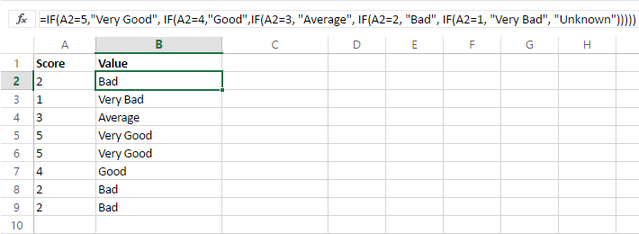
With the IF function you need to repeat the expression, so it takes more time to enter and looks longer.

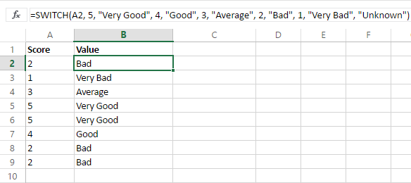
The same can be seen in the following example with the rating system where the Excel SWITCH function looks more compact.


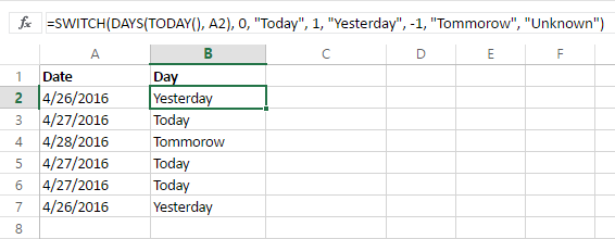
Let's see how SWITCH works in combination with other functions. Suppose, we have a number of dates and want to see at a glance if they refer to today, tomorrow, or yesterday. For this we add the TODAY function that returns the serial number of the current date, and DAYS that returns the number of days between two dates.
You can see that SWITCH works perfectly for this task.

With the IF function, the conversion needs some nesting and gets complex. So the chances of making an error are high.

Being underused and underestimated, Excel SWITCH is a really helpful function that lets you build conditional splitting logic.
 by
by
22 comments
Although it is better than a nested IF statement, SWITCH seems to be a roundabout way of simply using VLOOKUP to return the approriate value from a two-column table; the latter method would be a lot quicker than SWITCH especially if the lookup array is large, and considering you have to type the whole array into SWITCH anyway.
Why would I use SWITCH instead?
P.S. "tomorrow" has one "m" and two "r" :)
I'm manipulating a lot of data and I was wondering if there was a better way of to do things. I'm working with a big data frame in the background. This data frame has about 20 columns (height, lenght and thickness for example). All of these columns are dependant on the first columns that is the type of box that I use. For example, if I use box A it's height is 5 and it's lenght is 10. Coming back to my main sheet, I have drop-down list that includes all of boxes.I wan't my document to show me the height and lenght of my box when I choose box A for example. This would be quite easy with a few boxes as I would use the switch functions, but I have 400 types of boxes so it doesn't work.
Tintin: it's possibly a bit late now that it's December 2020, but you can simply use VLOOKUP to return the approriate values from your table ("data frame").
How can I write program in Excel for heart rate for adults child n infants
If rate in between 60 to 100 is normal
100 high
Hi Everyone, how do i write IF A1 has a value/symbol the delete value/symbol for B1 and C1
Thanks in advance
You are missing an element. You are using "HP" as the "there are no matches" result, but that means the string of values after " F2, " is missing something. There are 7 items and they must come in pairs, a value and its result, so one of them does not have its mate. Or I guess, there could be something stray/extra in there that needs removed. But basically, you need "F2", you need "HP", and everything else must be paird, sets of two things.
Also, it occurs to me looking at a problem above yours, that you may be loading it following the practice for IFS() in which you create a result for all previous things failing by using "TRUE,result for everything before this failed" or, in your case " TRUE(), "HP" ". But SWITCH() does NOT do this. So if it reaches that last pair, it evaluates TRUE() to be "TRUE", sees there is no match, and looks for something you want presented in the case of failure to match anything... but there is nothing, so it returns the error value.
BECAUSE it does not do things like IFS(), it has to let you present a value for "failure to find" as a single, explicit item. Notice that IFS does not let you do so, it requires a full pair, expression/result, that can ALWAYS succeed, like using TRUE or TRUE(). Weirdly for looking so similar, they act very differently "in the trenches."
So simply remove the " , TRUE() " entry and everything will be paired up and that final "HP" will be the default if nothing matches.
Having issues with the true part of this formula - results are showing #n/a instead of "HP"...
=SWITCH(F2, "998", "HI", "999", "HI", "485", "Ben", TRUE(), "HP")
very nice formula
New Formula, New Table, works great until the last: Anything over 39454 produces an N/A error.
=IFS(B17<0,C7,B17<716,C8,B17<2253,C9,B17<6957,C10,B17<13316,C11,B17<19920,C12,B17<35007,C13,B17<39453,C14)
IFS() does not let you state a single item at the end as a default result for everything preceding it failing their IF tests. (In this case, your " C14) " ending the formula.
You must use a final FULL clause, a pair of condition and result, at the end in order to get that as the "nothing passed its IF test, so result to this" result I think you wish.
However, it must ALWAYS succeed! Won't work well as a "catch-all" if it can also fail sometimes. Usual practice is to pick a function like TRUE() that will always result in success and pair it with your desired catch-all result:
So the end would look like this:
... ,B17<39453, TRUE(), C14)
and then it should work nicely.
(Compare that behavior with SWITCH() (see Col's post below). They look exceedingly like they work the same, but they are very different in the way the "everything else failed so return this result" clause is formed.)
I have the following formula, but Excel tells me it isn't valid. How do I fix this one?
=IF(ORD19>0,ORD19717,ORD192254,ORd196958,ORD1913317, ORD1919921,ORD1935008,ORD1939454),J27
It is supposed to be a tax table with the table from cells H20 to J27. The formulas in the J column work well individually, but I cannot get them to auto-figure in cell C17
This is cool indeed!
The Switch....Case statement is a staple in other programming languages; it was about time to have this important tool in Excel as well.
Thanks for letting the world know about this good news!
Trying to write the following function in excel. I have tried many combinations and just cant seem to get it to work
If A1>600, and A2500, and A2400, and A2<150, then A3=2
This would all be one long formula with a total of 21 possible combinations which would all change the value of the A3 cell. If anyone can help I would really appreciate it.
I have a data set that lists scores. the data set has three columns
win/loss sc1 sc2
L 100 90
W 101 98
If the result is "L" i need to transpose the sc1 and sc2...???
Im am looking for something simple and I know im over looking it. Using the IFs nestled. I want to type any number in one box, if that number is equal to or greater than 10 i want the output to be five, if it is equal to or less than 24.99 i want it to output nothing. I can get both parts to work but nestled together it wont work correctly
Thank you
Hi Donnie,
You should use the following formula:
=IF(AND(A1>=10, A1<=24.99), 5, "nothing")
Too nice sharing
Just in case cells C4 through F4 can contain numeric values other than 1 to 5 (or a blank cell) then you could use this.
=IF(COUNTIF(C4:F4,1)>0,1,IF(COUNTIF(C4:F4,2)>0,2,IF(COUNTIF(C4:F4,3)>0,3,IF(COUNTIF(C4:F4,4)>0,4,IF(COUNTIF(C4:F4,5)>0,5,"No Answer")))))
I'm sure there is probably a more elegant (simpler) way of doing this.
=IF(MIN(C4:F4)<=5,MIN(C4:F4),"No Answer")
How can I write an if statement for the following:
C4 thru F4 will either contain a 1, 2, 3, 4, or 5. If any of those cells have a 1, then G4 should be 1, if there isn't a 1, then if any of those cells have a 2, then G4 should be 2, if there isn't a 1 or 2, then if any of those cells have a 3, then G4 should be 3, if there isn't a 1, 2 or 3, then if any of those cells have a 4, then G4 should be 4, if there isn't a 1, 2, 3 or 4, then if any of those cells have a 5, then G4 should be 5. If there isn't a 1, 2, 3, 4, or 5 then G4 should say no answer.
Hi Wendy,
You should use the following formula:
=IF(OR(C4=1, D4=1,E4=1,F4=1), 1, IF(OR(C4=2, D4=2,E4=2,F4=2), 2, IF(OR(C4=3, D4=3,E4=3,F4=3), 3, IF(OR(C4=4, D4=4,E4=4,F4=4), 4, IF(OR(C4=5, D4=5,E4=5,F4=5), 5, "no answer")))))