Looking for a simple way to find duplicates in Google Sheets? How about 7 ways? :) That's all you need for numerous use cases :) I will show you how to use formula-free tools (no coding — promise!), conditional formatting and a few easy functions for avid formula fans.
No matter how often you use Google Sheets, chances are you have to deal with duplicated data. Such records may appear in one column or take up entire rows.
By the end of this article, you will know 1) how to remove duplicates, 2) count them, 3) highlight and 4) label with a status. I will show some formula examples and share different tools. One of them even finds and removes duplicates in your Google Sheets on schedule! Conditional formatting will also come in handy.
Just pick your poison and let's roll :)
Formula-free ways to find and remove duplicates in Google Sheets
Let's begin with the three most effortless solutions first. Two of them exist for the duplicate problem specifically.
1. Google Sheets native tool to remove duplicates
You probably already know that Google Sheets owns its small tool to remove duplicates. It has very few options, but it's super straightforward:
- Go to Data > Data cleanup tab and click Remove duplicates:

- Specify if your table has a header row and select all those columns that should be checked for duplicates:

- Click OK, and Google Sheets will find and delete duplicates from your table and say how many unique rows remain:

Though this may be enough for you, it's as far as this tool goes. Each time you need to deal with duplicates, you will have to run this utility manually. Also, this is all it does: delete duplicates. It neither counts them, nor color.
Luckily, Ablebits solved all these drawbacks in the Remove Duplicates add-on for Google Sheets.
2. Remove Duplicates add-on for Google Sheets
Remove Duplicates is an advanced version of the standard tool. But don't worry: advanced doesn't mean complicated. On the contrary, it's perfect for both spreadsheets beginners and pros.
Inside this toolkit, you'll have the Find duplicate or unique rows add-on. It offers 7 different ways to handle duplicates. And it doesn't just speed up the whole process — it knows how to automate it entirely.
Resides in your Google Sheets. Once you install it from the Google Workspace Marketplace, it will appear under the Extensions:

User-friendly process. As the standard Google Sheets tool, it also lets you select the range and columns to process but more elegantly :)
All settings fall into 4 user-friendly steps where you select:
- the range
- what to find: dupes or uniques
- the columns
- what to do with the found dupes or uniques
Directions all the way. You can even peek at special pictures within the tool so it's always clear what to do:

7 ways to handle duplicates. What's the point, you may think? Well, unlike the standard tool, this Remove Duplicates offers so much more for your Google Sheets:
- find duplicates or uniques with or without 1st occurrences
- highlight duplicates in Google Sheets
- add a label
- copy/move the results to a new sheet/spreadsheet or any specific place within your spreadsheet
- clear found values from cells
- delete duplicate rows from your Google Sheet completely

Just pick whatever way suits you best, select the options and let the add-on do the job.
Click the button below to install Remove Duplicates add-on for Google Sheets.
Video: How to remove duplicates in Google Sheets
Aside from this tool, this collection brings 5 more tools to find and remove duplicates in Google Sheets. This video will introduce them to you:
Make Google Sheets remove duplicates automatically
As icing on the cake, you will be able to save all the settings into scenarios and run them later on any table with just a click.
Or — even better — schedule those scenarios to kickstart automatically at a certain time daily:

Your presence is not necessary, and the add-on will delete duplicates automatically even when the file is closed or you're offline. To learn more about it, please visit this detailed tutorial.
Video: Remove Duplicates in Google Sheets automatically: by schedule
I encourage you to install Remove Duplicates from the Google Sheets store and poke around it.
You'll see how easily your Google Sheets will find duplicates, and remove or highlight duplicates and uniques without formulas in just a few clicks.
3. Find duplicates in Google Sheets with Pivot table
Google Sheets offers some other instruments to find duplicates.
Take Pivot table for example. It will sort of turn your data around and display it another way — without dupes! And it doesn't affect your original table. The latter works as a reference while the result is on a separate tab.
That result, by the way, will change dynamically depending on the settings you can tweak on the go.
Pivot table will help you count and remove duplicates in Google Sheets.
Example 1. How Pivot table counts duplicates in Google Sheets
- Go to Insert > Pivot table, specify your data range and a place for the pivot table:

- In the pivot table editor, add a column with your duplicates (Name in my example) for Rows and for Values.
If your column contains numeric records, pick COUNT as a summary function for Values to count duplicates in Google Sheets. If you have text, select COUNTA instead:

If you do everything correctly, the pivot table will feature each item from your list and get you the number of times it appears there:

As you can see, this pivot table shows that only blackberry and cherry reoccur in my data set.
Example 2. Remove duplicates in Google Sheets using Pivot table
To delete duplicates using the pivot table, you need to add the rest of your columns (2 in my example) as Rows for your pivot table:

You'll see the table with duplicate rows yet numbers will tell which of them reoccur in the original dataset:

Tip. If you don't need the numbers anymore, just close the Values box in the Pivot table by pressing the corresponding icon at its upper-right corner:

This is what your pivot table will look like eventually:

No duplicates, no extra calculations. Just unique records sorted out in one table.
Functions in Google Sheets that remove duplicates
Of course, you can also use formulas to find & remove duplicates in Google Sheets. Their main advantage is that your original table remains intact. The formulas identify duplicates and return the result to some other place in your Google Sheets. And based on the desired outcome, different functions do the trick.
1. Google Sheets UNIQUE to remove duplicates & original values
The UNIQUE function scans your data, deletes duplicates and returns exactly what its name says — unique values/rows.
Here's a small sample table where different rows reoccur:
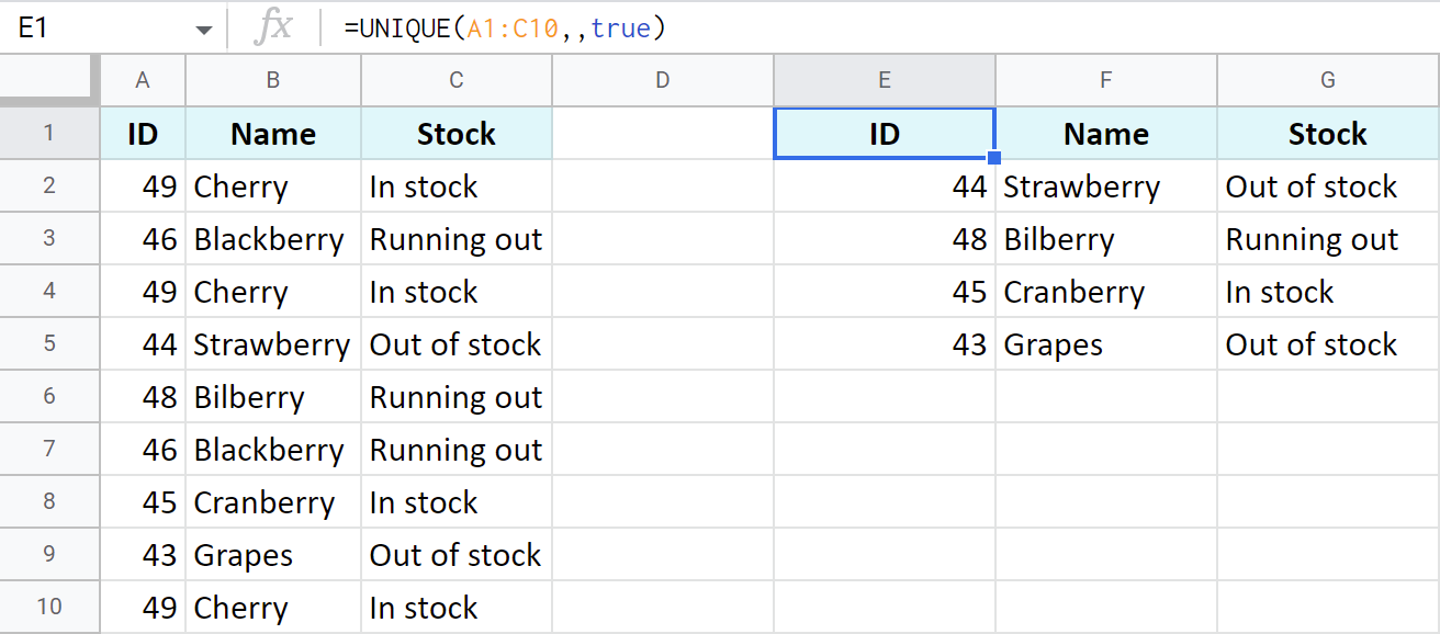
On one hand, you may need to remove all duplicate rows from this Google Sheets table and keep only the first entries. To do that, just enter the range for your data inside UNIQUE: This small formula returns all unique rows and all 1st occurrences ignoring 2nd, 3rd, etc. On the other hand, you may want to get only the "real" unique rows. By "real" I mean those that don't reoccur — not even once. So what do you do? Let's take a moment and look through all UNIQUE arguments: That last argument is your leverage here. Hence, to remove all duplicate rows from your Google Sheets completely (along with their 1st ), skip the second argument in the formula but add the third: See how the table on the right is much shorter? It's because Google Sheets UNIQUE found and removed duplicate rows as well as their 1st occurrences from the original table. Only unique rows remain now.
Example 1. Delete duplicate rows, keep the 1st occurrences
=UNIQUE(A1:C10)

Example 2. Delete all duplicate rows, even the 1st occurrences
=UNIQUE(A1:C10,,TRUE)

2. Google Sheets COUNTIF to find duplicates
If wasting cells with another dataset is not part of your plan, you can count duplicates in Google Sheets instead (and then delete them manually). It'll take just one extra column and the COUNTIF function will help.
Tip. If you're not familiar with this function, we have an entire blog post about it, feel free to take a look.
Example 1. Get total number of occurrences
Let's identify all duplicates with their 1st occurrences in Google Sheets and check the total number of each berry appearing on the list. I will enter the following formula in D2 and then copy it down the column:
=COUNTIF($B$2:$B$10,$B2)

Tip. To make this formula handle each row in the column automatically, wrap everything in ArrayFormula and change $B2 to $B2:$B10 (the whole column). Thus, you won't need to copy the formula down:

If afterwards you filter this dataset by the numbers, you will be able to see and even remove all duplicate rows from your Google Sheets table manually:

Example 2. Find and enumerate all duplicates in Google Sheets
In case the total number of occurrences is not your goal and you'd rather know whether this particular record in this particular row is the 1st, 2nd, etc entry, you'll need to make a slight adjustment to the formula.
Change the range from the entire column ($B$2:$B$10) to just one cell ($B$2:$B2).
Note. Pay attention to the use of absolute references.
=COUNTIF($B$2:$B2,$B2)

Now deleting duplicates from this Google Sheets table will be even easier because you'll be able to hide all entries but the 1st ones:

Example 3. Count duplicate rows in Google Sheets
All previous formulas count duplicates in a single Google Sheets column. But I know a formula that looks into all columns to identify duplicate rows.
In this case, COUNTIFS will suit you better. Just list every column of your table along with its corresponding criteria:
=COUNTIFS($A$2:$A$10,$A2,$B$2:$B$10,$B2,$C$2:$C$10,$C2)

Tip. There's another way available to calculate duplicates — without formulas. It involves a Pivot table and I described it above.
3. Google Sheets IF function to mark duplicates in a status column
Sometimes numbers are just not enough. Sometimes it's better to find duplicates and mark them in a status column. You can filter this column by statuses and remove those duplicates you no longer need.
Example 1. Find duplicates in 1 Google Sheets column
For this task, you will need the same COUNTIF function but this time wrapped in the IF function. Just like this:
=IF(COUNTIF($B$2:$B$10,$B2)>1,"Duplicate","Unique")

Let's see what happens in this formula:
- First, COUNTIF searches the entire column B for the berry from B2. Once found, it sums them up.
- Then, IF checks this total, and if it's greater than 1, it says Duplicate, otherwise, Unique.
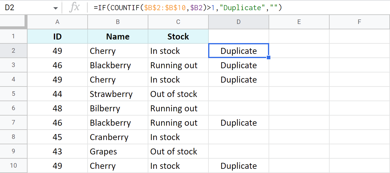
Of course, you can make the formula to return your own statuses, for example, find & identify only duplicates in your Google Sheets data:
=IF(COUNTIF($B$2:$B$10,$B2)>1,"Duplicate","")

Tip. As soon as you find these duplicates, you can filter the table by the status column. This way lets you hide repeated or unique records, and even select entire rows & delete these duplicates from your Google Sheets completely:

Example 2. Identify duplicate rows
Similarly, you can mark absolute duplicate rows — rows where all records in all columns appear several times in the table:
- Start with the same COUNTIFS from before — the one that scans each column for its first value and counts only those rows where all 3 records in all 3 columns repeat themselves:
=COUNTIFS($A$2:$A$10,$A2,$B$2:$B$10,$B2,$C$2:$C$10,$C2) - Then enclose that formula in IF. It checks the number of repeated rows and if it exceeds 1, the formula names the row as a duplicate:
=IF(COUNTIFS($A$2:$A$10,$A2,$B$2:$B$10,$B2,$C$2:$C$10,$C2)>1,"Duplicate","")

Now this table has only 2 dupes. Even though cherry occurs 3 times in a table, only two of them have all 3 columns identical.
Example 3. Find duplicate rows, ignore the 1st entries
To ignore the 1st occurrence and mark only the 2nd and the other ones, refer to the first cells of the table instead of the entire columns:
=IF(COUNTIFS($A$2:$A2,$A2,$B$2:$B2,$B2,$C$2:$C2,$C2)>1,"Duplicate","")

Tip. If you are using Microsoft Excel, the following examples might be helpful: How to find duplicates in Excel.
Identify and highlight duplicates in Google Sheets using conditional formatting
Did you know that you can spot duplicates in your table at a single glance? All you need to do is highlight duplicates in Google Sheets. Conditional formatting will help you with this.
Tip. Visit this tutorial for more formulas to highlight duplicates in Google Sheets.
Here's what you need to do:
- Open conditional formatting settings: Format > Conditional formatting.
- Make sure that the Apply to range field contains the range of cells where you want to highlight duplicates. For this example, let me start with column B.
- In Format rules pick Custom formula is and enter the same COUNTIF that I introduced above:
=COUNTIF($B$2:$B$10,$B2)>1
Once it locates records that appear at least twice in column B, they will be colored with a hue of your choice:

Another option would be to highlight duplicate rows. Simply adjust the range to apply the rule to multiple columns:

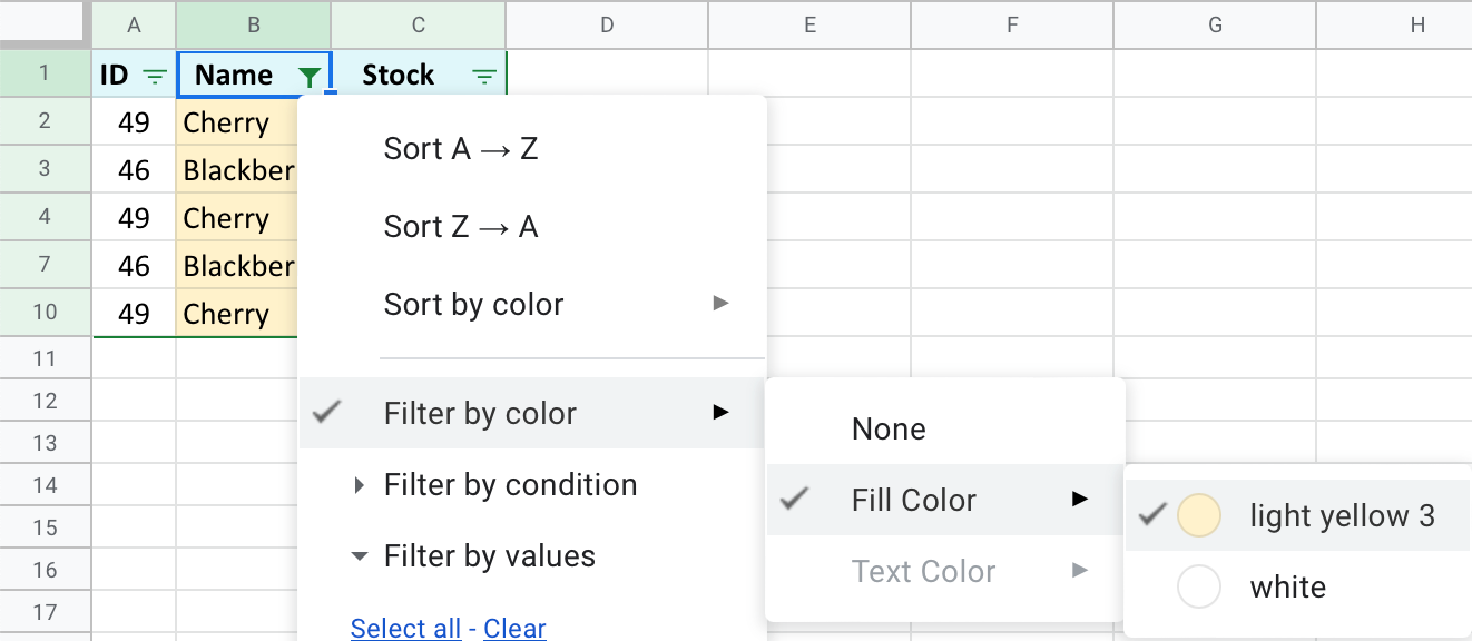
Tip. Once you highlight duplicates in your Google Sheets, you can filter the data by color:
- On one hand, you can filter the column so that only cells with the white fill color remain visible. This way, you will delete duplicates from the view:

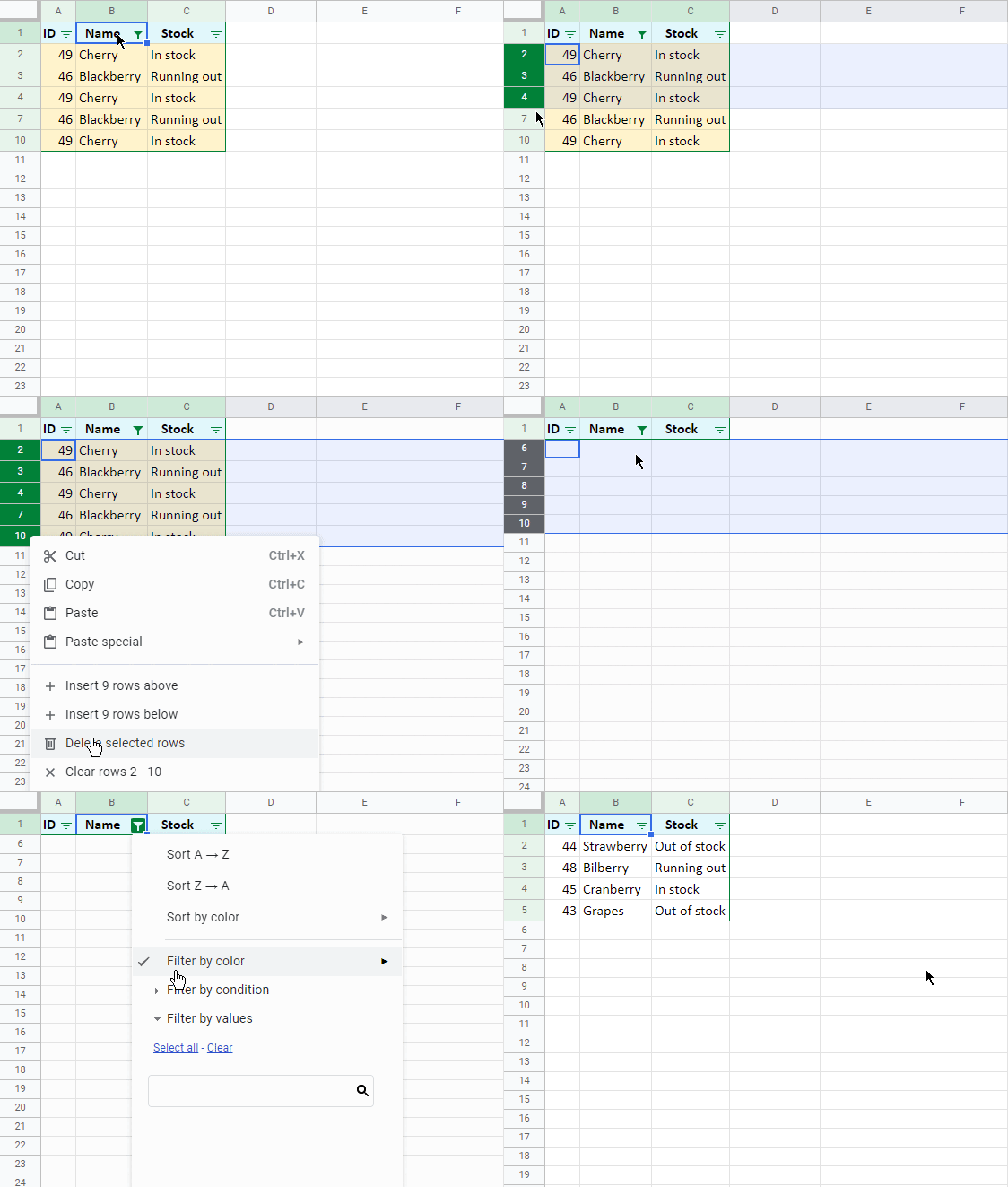
- On the other hand, you can keep only colored cells visible:

and then select these rows and delete these duplicates from your Google Sheets completely:

Spreadsheet with formula examples
Find & remove duplicates in Google Sheets (make yourself a copy to practice)
 by
by
21 comments
I'm trying to get duplicate names figured out on a sheet, however the cells don't match exactly. I'm wondering if there's a way I can find duplicates if the cells don't match exactly?
Hello Taylor,
To look for partial matches using formulas, you need to use wildcard characters. Here are a few examples: with VLOOKUP and COUNTIF.
Or use REGEXEXTRACT.
Alternatively, you can try this free add-on: Find Fuzzy Matches
I want to delete duplicates just like this but instead of keeping one unique value I want to have the unique value and one of its duplicates to stay and the rest of the duplicates deleted. To leave only two. Is there a way to do that.
Hello Cabot,
Yes, there is. Use this tool and on its second step choose to find Duplicates + 1st occurrences (or Uniques + 1st occurrences, I'm just not sure what you meant exactly. Pick the one that suits you best.).
i have number of website list but i want to remove duplicate website with using prefix of website name .
Hello Anjali,
So you need to remove duplicates but only for certain websites, right?
I have a data set in a Google Sheet that captures employee time off requests for vacation, sick days, etc. The data includes a Start Date column and an End Date column. For example, someone is requesting vacation from 1/1/2023 to 1/15/2023. I am trying to identify dupes (i.e. overlapping dates). For example, if that same person enters another record later on for vacation from 1/10/2023 to 1/15/2023, we know that is impossible - they can't be off "twice" on the same days.
What is the best way to capture those types of duplicates? It's not just the values on the columns, but the data range in between.
Thanks,
Ken
Hello KenW,
For me to be able to help you better, please share a small sample spreadsheet with us (support@apps4gs.com) with 2 sheets: (1) a copy of your source data (2) the result you expect to get. (The result sheet is of great importance as it gives us a better understanding than any text description.) I kindly ask you to shorten the tables to 10-20 rows. If you have confidential information there, you can replace it with some irrelevant data, just keep the format.
Note. We keep that Google account for file sharing only and don't monitor its Inbox. Please do not email there. Once you share the file, just confirm by replying to this comment.
I'll look into it and try to help.
Hi, I want duplicate entries to be sorted in another column, how can I do it? Like this:
A B C D
Items Duplicates Count
from column A
Apple Apple 3
Banana Cherry 2
Cherry Grapes 2
Apple
Grapes
Mango
Cherry
Apple
Grapes
I want ONLY duplicates to be pulled into column C and ignore unique data. Please help thank u!
Sorry, the sample table messed up.
Hello Jek,
For me to be able to help you better, please share your sample spreadsheet with us (support@apps4gs.com) with 2 sheets: (1) a copy of your source data (2) the result you expect to get. I kindly ask you to shorten the tables to 10-20 rows.
Note. We keep that Google account for file sharing only and don't monitor its Inbox. Please do not email there. Once you share the file, just confirm by replying to this comment.
I'll look into it and try to help.
Thank you! Very helpful!
You're most welcome, Alexandre! Appreciate your feedback :)
Hey again!
Tried this one as well:
=arrayformula(IF(COUNTIFS(arrayformula($A$2:$A2&$G$2:$G2),$A$2:$A2,$A2&$G$2:$G2,$G2)>1,"Duplicate","Pass"))
It doesn't array the whole column, only the first one.
2nd try:
Added to a range
=arrayformula(IF(COUNTIFS(arrayformula($A$2:$A&$G$2:$G),$A$2:$A,$A2&$G$2:$G,$G2)>1,"Duplicate","Pass"))
Then array works, but then all the values are fail aka "Pass"
Hi Kevin,
Could you please share an editable copy of your sheet with your formula with us (support@apps4gs.com)? If you have confidential information there, you can replace it with some irrelevant data, just keep the format. I'll look into it and try to help.
Note. We keep that Google account for file sharing only and don't monitor its Inbox. Please do not email there. Once you share the file, just confirm by replying to this comment.
Hey!
Section "Example 3. Find duplicate rows, ignore the 1st entries"
Is it possible to make it work with an arrayformula?
=arrayformula(if(A2:A2="","",if(COUNTIF(ArrayFormula($A2:A2&$G2:G2),$A$2:$A2&$G$2:$G2)>1,"Duplicate","")))
doesn't seems to work. arrayformula needs a range, so no hope here?
Hi Kevin,
Could you please share an editable copy of your sheet with your formula with us (support@apps4gs.com)? If you have confidential information there, you can replace it with some irrelevant data, just keep the format. I'll look into it and try to help.
Note. We keep that Google account for file sharing only and don't monitor its Inbox. Please do not email there. Once you share the file, just confirm by replying to this comment.
...and fixed it :)
=COUNTIF($A$1:$A;SUBSTITUTE($A$1:$A;" ";""))>1
Thanks any way :) Hope this helps others who have the same problem.
Bora
Hello Bora,
Glad to know you've found the formula that works for you :) Thank you for sharing!
BTW, you can also try TRIM instead of SUBSTITUTE. It removes all leading & trailing spaces and reduces those in-between words to one.
Thank you Sister :)
You're most welcome, Taj!