The tutorial shows a few quick ways to flip tables in Excel vertically and horizontally preserving the original formatting and formulas.
Flipping data in Excel sounds like a trivial one-click task, but surprisingly there is no such built-in option. In situations when you need to reverse the data order in a column arranged alphabetically or from smallest to largest, you can obviously use the Excel Sort feature. But how do you flip a column with unsorted data? Or, how do you reverse the order of data in a table horizontally in rows? You will get all answers in a moment.
Flip data in Excel vertically
With just a little creativity, you can work out a handful of different ways to flip a column in Excel: by using inbuilt features, formulas, VBA or special tools. The detailed steps on each method follow below.
How to flip a column in Excel
The reverse the order of data in a column vertically, perform these steps:
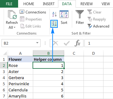
- Add a helper column next to the column you want to flip and populate that column with a sequence of numbers, starting with 1. This tip shows how to have it done automatically.
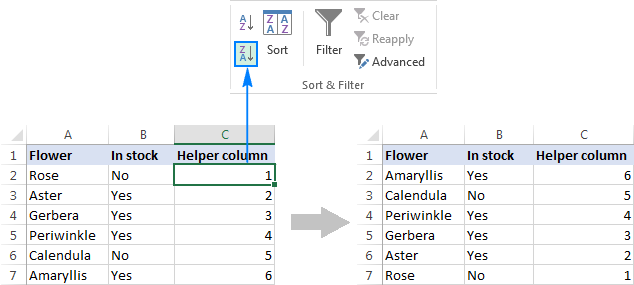
- Sort the column of numbers in descending order. For this, select any cell in the helper column, go to the Data tab > Sort & Filter group, and click the Sort Largest to Smallest button (ZA).

As shown in the screenshot below, this will sort not only the numbers in column B, but also the original items in column A, reversing the order of rows:

Now you can safely delete the helper column since you do not need it any longer.
Tip: How to quickly fill a column with serial numbers
The fastest way to populate a column with a sequence of numbers is by using the Excel AutoFill feature:
- Type 1 into the first cell and 2 into the second cell (cells B2 and B3 in the screenshot below).
- Select the cells where you've just entered the numbers and double-click the lower right corner of the selection.

That's it! Excel will autofill the column with serial numbers up to the last cell with data in the adjacent column.
How to flip a table in Excel
The above method also works for reversing the data order in multiple columns:

Sometimes (most often when you select the whole column of numbers prior to sorting) Excel might display the Sort Warning dialog. In this case, check the Expand the selection option, and then click the Sort button.

Tip. If you'd like to switch rows and columns, use the Excel TRANSPOSE function or other ways to transpose data in Excel.
How to flip columns in Excel using a formula
Another way to flip a column upside down is by using this generic formula:
For our sample data set, the formula goes as follows:
=INDEX($A$2:$A$7,ROWS(A2:$A$7))
…and reverses column A impeccably:
At the heart of the formula is the INDEX(array, row_num, [column_num]) function, which returns the value of an element in array based on the row and/or column numbers you specify. In the array, you feed the entire list you want to flip (A2:A7 in this example). The row number is worked out by the ROWS function. In its simplest form, ROWS(array) returns the number of rows in array. In our formula, it's the clever use of the relative and absolute references that does the "flip column" trick: In other words, ROWS creates a kind of decrementing counter for INDEX so that it moves from the last item toward the first item. Tip: How to replace formulas with values Now that you have two columns of data, you may want to replace formulas with calculated values, and then delete an extra column. For this, copy the formula cells, select the cells where you'd like to paste the values, and press Shift+F10 then V, which is the fastest way to apply Excel's Paste Special > Values option.
For more information, please see How to replace formulas with values in Excel.
How this formula works

How to flip columns in Excel with VBA
If you have some experience with VBA, you can use the following macro to reverse the data order vertically in one or several columns:
How to use the Flip Columns macro
- Open the Microsoft Visual Basic for Applications window (Alt + F11).
- Click Insert > Module, and paste the above code in the Code window.
- Run the macro (F5).
- The Flip Columns dialog pops up prompting you to select a range to flip:

You select one or more columns using the mouse, not including the column headers, click OK and get the result in a moment.
To save the macro, be sure to save your file as an Excel macro-enabled workbook.
How to flip data in Excel preserving formatting and formulas
With the above methods, you can easily reverse the data order in a column or table. But what if you not only wish to flip values, but cell formats too? Additionally, what if some data in your table is formula-driven, and you want to prevent formulas from being broken when flipping columns? In this case, you can use the Flip feature included with our Ultimate Suite for Excel.
Supposing you have a nicely formatted table like shown below, where some columns contain values and some columns have formulas:

You are looking to flip the columns in your table keeping both formatting (grey shading for rows with zero qty.) and correctly calculated formulas. This can be done in two quick steps:
- With any cell in your table selected, go to the Ablebits Data tab > Transform group, and click Flip > Vertical Flip.

- In the Vertical Flip dialog window, configure the following options:
- In the Select your range box, check the range reference and make sure the header row is not included.
- Select the Adjust cell references option and check the Preserve formatting box.
- Optionally, choose to Create a back up copy (selected by default).
- Click the Flip button.

Done! The order of data in the table is reversed, the formatting is kept, and cell references in the formulas are appropriately adjusted:

Flip data in Excel horizontally
So far in this tutorial, we have flipped columns upside down. Now, let's look at how to reverse data order horizontally, i.e. flip a table from left to right.
How to flip rows in Excel
As there is no option to sort rows in Excel, you'll need to first change rows to columns, then sort columns, and then transpose your table back. Here are the detailed steps:
- Use the Paste Special > Transpose feature to convert columns to rows. As the result, your table will undergo this transformation:

- Add a helper column with numbers as in the very first example, and then sort by the helper column. Your intermediate result will look something like this:

- Use Paste Special > Transpose one more time to rotate your table back:

Note. If your source data contains formulas, they may be broken during the transpose operation. In this case, you will have to restore the formulas manually. Or you can use the Flip tool included in our Ultimate Suite and it will adjust all the references for you automatically.
Reverse data order horizontally with VBA
Here is a simple macro that can quickly flip data in your Excel table horizontally:
To add the macro to your Excel workbook, please follow these steps. As soon as you run the macro, the following dialog window will show up, asking you to select a range:

You select the entire table, including the header row, and click OK. In a moment, the data order in rows in reversed:

Flip data in rows with Ultimate Suite for Excel
Similarly to flipping columns, you can use our Ultimate Suite for Excel to reverse the order data in rows. Just select a range of cells you want to flip, go to the Ablebits Data tab > Transform group, and click Flip > Horizontal Flip.

In the Horizontal Flip dialog window, choose the options appropriate for your data set. In this example, we are working with values, so we choose Paste values only and Preserve Formatting:

Click the Flip button, and your table will be reversed from left to right in the blink of an eye.
This is how you flip data in Excel. I thank you for reading and hope to see you on our blog next week!
 by
by
15 comments
Hello dear Team,
I need your help on that matter,
1. HBC 1920 the result should be 1920 HBC
2. HBC 1760 the result should be 1760 HBC
3. P-296800 the result should be -296800 P
Thanks a lot in advance please.
Please help sir,
Hi!
Unfortunately, I cannot solve your problem with a formula. Your cells have a different data pattern.
So Kindly check the Sr.No. 1&2 are the same pattern,
so may be the formula for this.
Split the text string in the cell using this instruction: How to split text string in Excel by comma, space, character or mask.
Then combine text strings as described here: CONCATENATE in Excel: combine text strings, cells and columns.
Try this formula:
=MID(A1,SEARCH(" ",A1)+1,10)&""&LEFT(A1,SEARCH(" ",A1)-1)
Thanks a lot Sir,
This is working very well.
"As there is no option to sort rows in Excel, ..."
In fact, there is an easier method for sorting rows horizontally:
1. Insert a helper-row , say e.g. row 1, and fill it with numbers 1, 2, ...
2. Select the whole range, including the first (helper-) row
3. On Home tab go to Editing group, Select "Custom-Sort".
4. Important: Press "Options" button, and check the box labeled "Sort left to right", then press OK.
5. In sort properties, select sort by Row 1, order descending (large to small).
6. Press OK.
thanks
Very nice Article,
How we can more than one column flip to use index formula?
Hello!
There are many ways in this article how to transpose multiple columns. This cannot be done using the INDEX function.
Indeed, a very good tutorial! It provides user-friendly information without going overboard with jargon and technical terms. By all means, the raw basics are outlined in this nicely-written article, using some text and images. I always encourage my students to refer to your sites for speedy answers to Excel questions.
Keep the great work up, Svetlana!
Dear Dr. Choueiri,
Thank you very much for your encouraging comment!
To flip horizontally, you can also simply transpose first, then sort A-Z (if necessary add column with numbers first to use to), then transpose back. Done.
excelent solution
Hi Roman,
Wonderful idea, thank you for sharing! Hope you won't mind that I included this method in the tutorial and included a few visuals to better convey the steps. Just one caveat: if the source data contains formulas, they may get broken during the transpose process.