The tutorial shows how to freeze cells in Excel to keep them visible while you navigate to another area of the worksheet. Below you will find the detailed steps on how to lock a row or multiple rows, freeze one or more columns, or freeze column and row at once.
When working with large datasets in Excel, you may often want to lock certain rows or columns so that you can view their contents while scrolling to another area of the worksheet. This can be easily done by using the Freeze Panes command and a few other features of Excel.
How to freeze rows in Excel
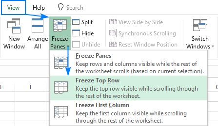
Freezing rows in Excel is a few clicks thing. You just click View tab > Freeze Panes and choose one of the following options, depending on how many rows you wish to lock:
- Freeze Top Row - to lock the first row.
- Freeze Panes - to lock several rows.
The detailed guidelines follow below.
How to freeze top row in Excel
To lock top row in Excel, go to the View tab, Window group, and click Freeze Panes > Freeze Top Row.
This will lock the very first row in your worksheet so that it remains visible when you navigate through the rest of your worksheet.

You can determine that the top row is frozen by a grey line below it:

How to freeze multiple rows in Excel
In case you want to lock several rows (starting with row 1), carry out these steps:
- Select the row (or the first cell in the row) right below the last row you want to freeze.
- On the View tab, click Freeze Panes > Freeze Panes.
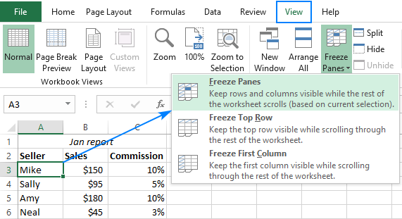
For example, to freeze top two rows in Excel, we select cell A3 or the entire row 3, and click Freeze Panes:

As the result, you'll be able to scroll through the sheet content while continuing to view the frozen cells in the first two rows:

Notes:
- Microsoft Excel allows freezing only rows at the top of the spreadsheet. It is not possible to lock rows in the middle of the sheet.
- Make sure that all the rows to be locked are visible at the moment of freezing. If some of the rows are out of view, such rows will be hidden after freezing.
How to freeze columns in Excel
Freezing columns in Excel is done similarly by using the Freeze Panes commands.
How to lock the first column
To freeze the first column in a sheet, click View tab > Freeze Panes > Freeze First Column.
This will make the leftmost column visible at all times while you scroll to the right.

How to freeze multiple columns in Excel
In case you want to freeze more than one column, this is what you need to do:
- Select the column (or the first cell in the column) to the right of the last column you want to lock.
- Go to the View tab, and click Freeze Panes > Freeze Panes.
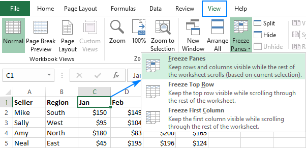
For example, to freeze the first two columns, select the whole column C or cell C1, and click Freeze Panes:

This will lock the first two columns in place, as indicated by the thicker and darker border, enabling you to view the cells in frozen columns as you move across the worksheet:

Notes:
- You can only freeze columns on the left side of the sheet. Columns in the middle of the worksheet cannot be frozen.
- All the columns to be locked should be visible, any columns that are out of view will be hidden after freezing.
How to freeze rows and columns in Excel
Besides locking columns and rows separately, Microsoft Excel lets you freeze both rows and columns at the same time. Here's how:
- Select a cell below the last row and to the right of the last column you'd like to freeze.
- On the View tab, click Freeze Panes > Freeze Panes.
Yep, it's that easy :)
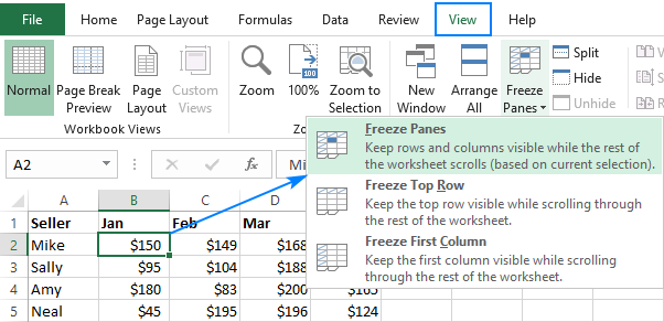
For example, to freeze top row and first column in a single step, select cell B2 and click Freeze Panes:

This way, the header row and leftmost column of your table will always be viewable as you scroll down and to the right:

In the same fashion, you can freeze as many rows and columns as you want as long as you start with the top row and leftmost column. For instance, to lock top row and the first 2 columns, you select cell C2; to freeze the first two rows and the first two columns, you select C3, and so on.
How to unlock rows and columns in Excel
To unlock frozen rows and/or columns, go to the View tab, Window group, and click Freeze Panes > Unfreeze Panes.

Freeze Panes not working
If the Freeze Panes button is disabled (greyed out) in your worksheet, most likely it's because of the following reasons:
- You are in cell editing mode, for example entering a formula or editing data in a cell. To exit cell editing mode, press the Enter or Esc key.
- Your worksheet is protected. Please remove the workbook protection first, and then freeze rows or columns.
Other ways to lock columns and rows in Excel
Apart from freezing panes, Microsoft Excel provides a few more ways to lock certain areas of a sheet.
Split panes instead of freezing panes
Another way to freeze cells in Excel is to split a worksheet area into several parts. The difference is as follows:
Freezing panes allows you to keep certain rows or/and columns visible when scrolling across the worksheet.
Splitting panes divides the Excel window into two or four areas that can be scrolled separately. When you scroll within one area, the cells in the other area(s) remain fixed.

To split Excel's window, select a cell below the row or to the right of the column where you want the split, and click the Split button on the View tab > Window group. To undo a split, click the Split button again.
Use tables to lock top row in Excel
If you'd like the header row to always stay fixed at the top while you scroll down, convert a range to a fully-functional Excel table:

The fastest way to create a table in Excel is by pressing the Ctl + T shortcut. For more information, please see How to make a table in Excel.
Print header rows on every page
In case you'd like to repeat top row or rows on every printed page, switch to the Page Layout tab, Page Setup group, click the Print Titles button, go to the Sheet tab, and select Rows to repeat at top. The detailed instructions can be found here: Print row and column headers on every page.
That's how you can lock a row in Excel, freeze a column, or freeze both rows and columns at a time. I thank you for reading and hope to see you on our blog next week!
 by
by
4 comments
How can I freeze multiple row and column at a time?
Hi Dheeraj,
Simply select a cell below the last row and to the right of the last column you'd like to freeze, and then click Freeze Panes > Freeze Panes.
Please see the "How to freeze rows and columns in Excel" section for the detailed steps with screenshots.
The freeze panes only freezes the top row now (excel 2016) so the program is getting worse.
You have to use Freeze panes instead of freeze first row and coloumn.