Dates are an inevitable part of Google Sheets. And like many other concepts of spreadsheets, they require a bit of learning.
In this tutorial, you will find out how Google stores dates and how you can format them for your better convenience. Some date formats are offered to you by spreadsheets while others should be created from scratch. There are even a couple of handy functions for the task.
I also describe a couple of ways to convert your dates to numbers and text if necessary.
How Google Sheets formats dates
First things first: before any activities related to dates in spreadsheets, it's crucial to understand the core principles of how dates work.
For its internal database, Google Sheets stores all dates as integer numbers. Not sequences of a day, month, and year as we got used to seeing, but simple integers:
- 1 for December 31, 1899
- 2 for January 1, 1900
- 102 for April 11, 1900 (100 days after January 1, 1900)
- and so on.
Unlike Excel that cannot store dates as negative numbers, in Google, for dates prior to December 31, 1899, the numbers will be negative:
- -1 for December 29, 1899
- -2 for December 28, 1899
- -102 for September 19, 1899
- etc.
Regardless of how Google Sheets formats dates for you to see in cells, spreadsheets always store them as integers. It's an automatic Google Sheets date format that helps to treat dates correctly.
Tip. The same goes for time units – they are merely decimals for your table:
- .00 for 12:00 AM
- .50 for 12:00 PM
- .125 for 3:00 AM
- .573 for 1:45 PM
- etc.
A date paired with time is kept as an integer with decimal places:
- 31,528.058 is April 26, 1986, 1:23 AM
- 43,679.813 is August 2, 2019, 7:30 PM
Change date format in Google Sheets to another locale
Another important thing to keep in mind is your spreadsheet locale.
The locale is what presets your Google Sheets date format based on your region. Thus, if you're currently in the US, 06-Aug-2019 will be put as 8/6/2019 in your sheet, while for the UK it'll be 6/8/2019.
To ensure the correct calculations, it's vital to have the correct locale set, especially if the file was created in another country:
- Go to File > Settings in the Google Sheets menu.
- Find Locale under the General tab and pick the desired location from the drop-down list:
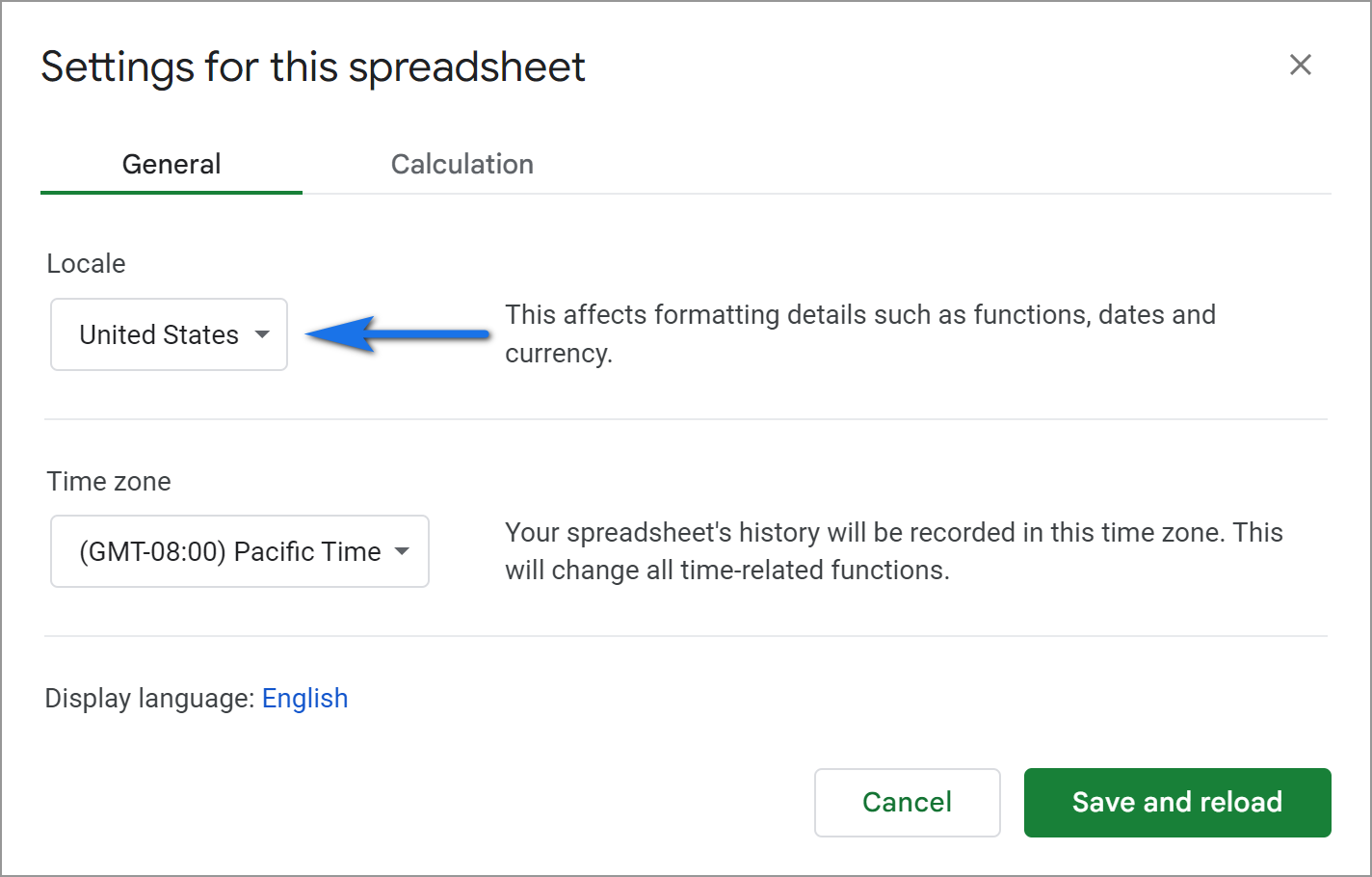
Tip. As a bonus, you can also specify your time zone here to record your file history in it.
Note. The locale doesn't change the language of your Sheets. However, the date formatting will be applied to the entire spreadsheet. Everyone who works with it will see the changes, no matter their place on the globe.
How to change date format in Google Sheets
If dates in your tables are formatted inconsistently or all you can see is strange sets of numbers instead, don't panic. You simply need to change the date format in your Google Sheets using built-in instruments.
Default Google Sheets date format
- Select all cells you'd like to format.
- Go to Format > Number in the spreadsheet menu and pick Date to see the date only or Date time to get both date and time in a cell:
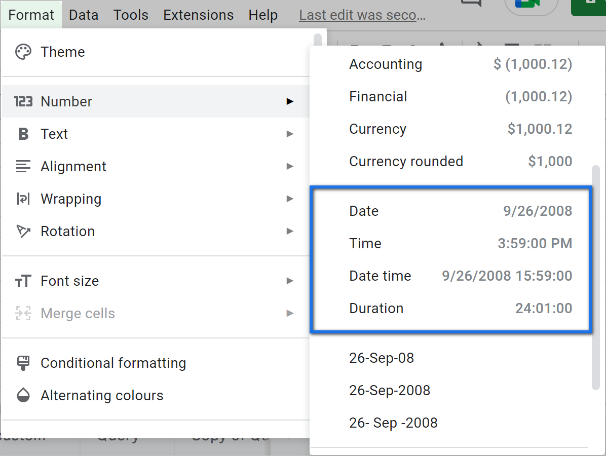
The integers successfully turn into the format that you'll recognize at a glance. These are default Google Sheets date formats:

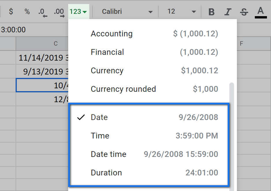
Tip. You can find the same formats if you click on the 123 icon on the spreadsheet toolbar:
Custom date formats
If you don't like how Google Sheets formats dates by default, I won't blame you. Luckily, there's plenty of room to improvise thanks to custom date formats.
You can access them from the same Google Sheets menu: Format > Number > Custom date and time:
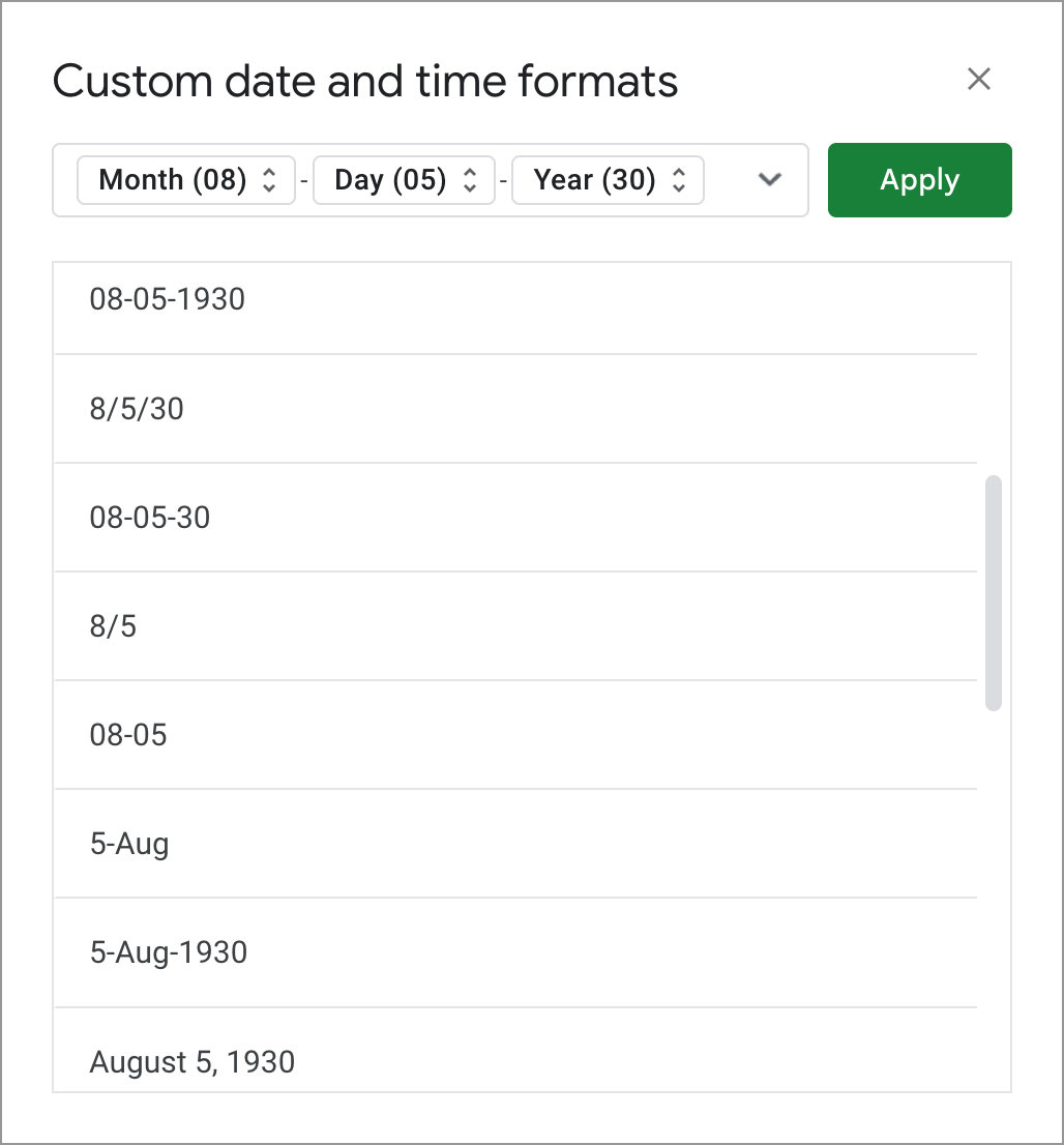
You will see the window with lots of different custom date formats available. Whichever one you chose and apply, your dates will look the same:

If you're still unhappy with the appearance of your dates, you can tailor your own custom date format:
- Select the cells you want to format.
- Go to Format > Number > Custom date and time.
- Place the cursor into the field at the top that contains the date units and delete everything with your Backspace or Delete keys:
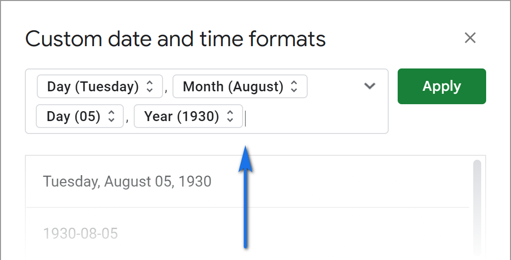
- Click the arrow to the right of the field and pick the unit you'd like to have first. Don't forget to type the separator afterwards.
Repeat till all the necessary units are added (no worries, you'll be able to add or remove them later):

- Notice that each unit has double arrows to its right. Click them and you'll be able to adjust the exact way to display the value.
Here's what I can choose for Day:

This way, you can edit all values, insert additional and delete obsolete ones. You are free to separate the units with various characters including commas, slashes, and dashes.
- Once you're ready, click Apply.
Here's what format I've created and how my dates look now:
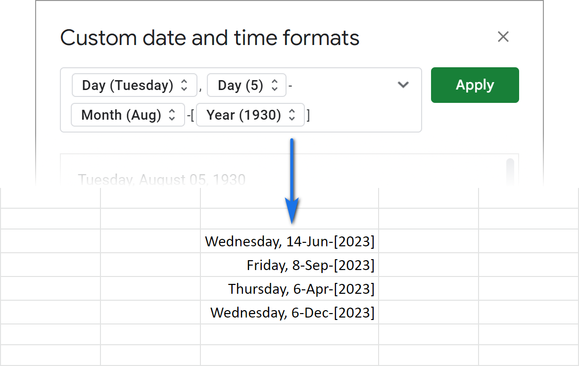
QUERY function for Google Sheets to format dates
There's one more way to change date format in Google Sheets – with a formula, of course. Since this is not the first time of me showing QUERY to you, I'm starting to think of it as a real cure-all for spreadsheets. :)
I have an example table where I track the shipment of a few orders:
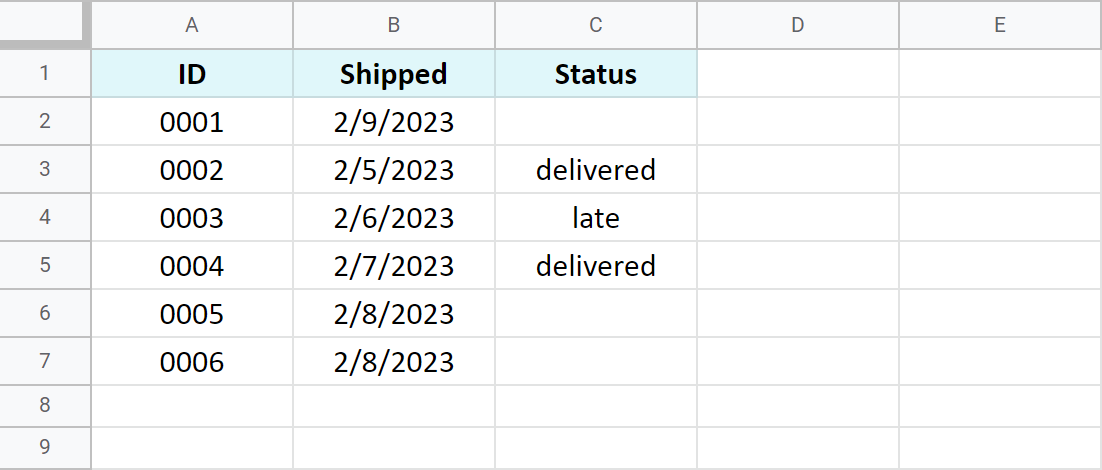
I want to change the date format in column B. Here's my QUERY formula:
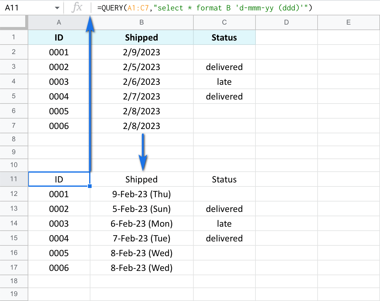
=QUERY(A1:C7,"select * format B 'd-mmm-yy (ddd)'")
- first, I specify the range of my entire table – A1:C7
- then I'm asking the formula to return all columns – select *
- and at the same time re-format column B the way I put into the formula – format B 'd-mmm-yy (ddd)'
The formula works like a charm. It returns my entire table and changes date format in column B:
As you may have noticed, to change the date format via the formula, I used special codes that represent different looks of days, months, and years. If you're not familiar with them, here's a list of these codes for dates:
| Code | Description | Example |
| d | Day without a leading zero for 1-9 | 7 |
| dd | Day with a leading zero for 1-9 | 07 |
| ddd | Day as an abbreviation | Wed |
| dddd | Day as a full name | Wednesday |
| m (if not preceded or followed by hours or seconds) |
Month without a leading zero | 8 |
| mm (if not preceded or followed by hours or seconds) |
Month with a leading zero | 08 |
| mmm | Month as an abbreviation | Aug |
| mmmm | Month as a full name | August |
| mmmmm | First letter of the month | A |
| y or yy |
Two digit year | 19 |
| yyy or yyyy |
Full numeric year | 2019 |
Tip. If you'd like to supply your date format with time as well, you need to add codes for time units. You will find the full list of time codes in this guide.
Using these codes, you can format the dates in so many ways:
- Get the hold of the year, month, or day only:
=QUERY(A1:C7,"select * format B 'yyyy'")
- Return the day, month, and the day of the week:
=QUERY(A1:C7,"select * format B 'dd mmmm, dddd'")
By the way, what date format have you got used to? :)
Google Sheets: convert date to number
In case you need to see numbers instead of dates, one of the methods below will be useful.
Convert date to number by changing the format
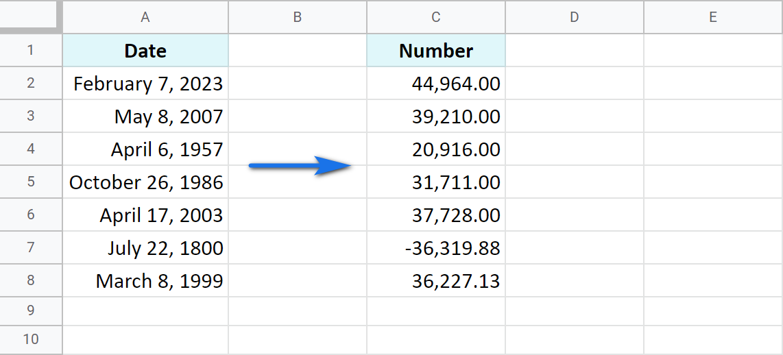
- Select those cells with dates that you want to convert to numbers.
- Go to Format > Number and this time pick Number among other options.
- Voila – all selected dates have turned into numbers that represent them:
DATEVALUE function for Google Sheets
Another way for Google Sheets to convert date to number is by using the DATEVALUE function:
where date_string represents any date in the known for spreadsheets format. The date should be put in double-quotes.
For example, I want to convert August 10, 2023 to a number. All the formulas below will return the same result: 45148.
=DATEVALUE("August 10, 2023")
=DATEVALUE("2023-8-10")
=DATEVALUE("8/10/2023")

Tip. If you're not sure whether Google Sheets understands the format you're about to enter, try typing the date into another cell first. If the date is recognized, it'll be aligned to the right.
You can also fill your cells with dates in one column, and then reference them in your formulas in another column:
=DATEVALUE(A2)
Google Sheets: convert date to text
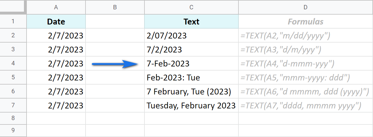
Converting dates to text in spreadsheets is the task for the TEXT function:
- number – regardless of what number, date, or time you give to the function, it will return it as text.
- format – the text will be formatted the way you specify in the formula.
Tip. To set the format correctly, use the same codes as you did for the QUERY function.
The real-data formula may look like this:
=TEXT("2/7/2023","YYYY-MM-DD")
Here's how I converted my date – 2/7/2023 - to text and changed the format at the same time:
Google Sheets: convert text to date
Sometimes your dates may appear in a way that Google Sheets doesn't understand at all. And it doesn't really matter whether they are imported or you just fancy a certain view:
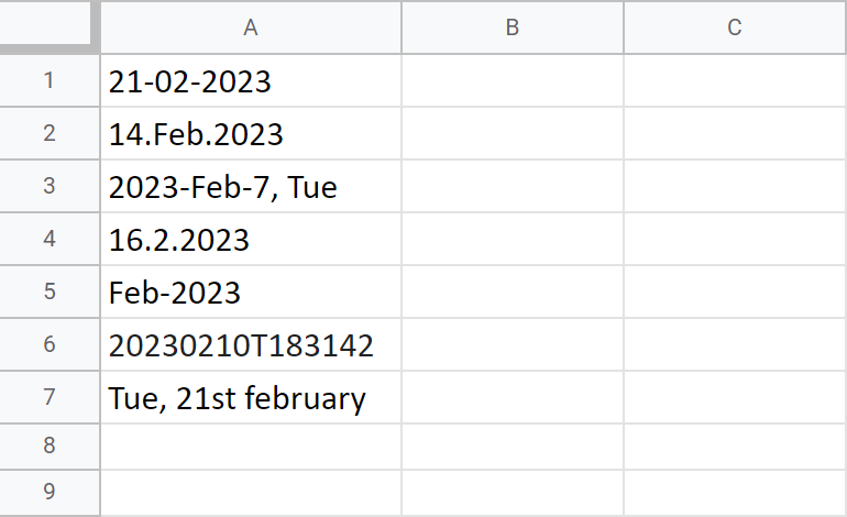
Unless you specify a custom format for each cell or change the locale of your spreadsheet, these dates will be formatted as text by default. You won't be able to use them in formulas or other calculations.
But here's the easiest solution for your Google Sheets: convert text to dates using the Power Tools add-on.
It's literally a single radio button among other convert tools.
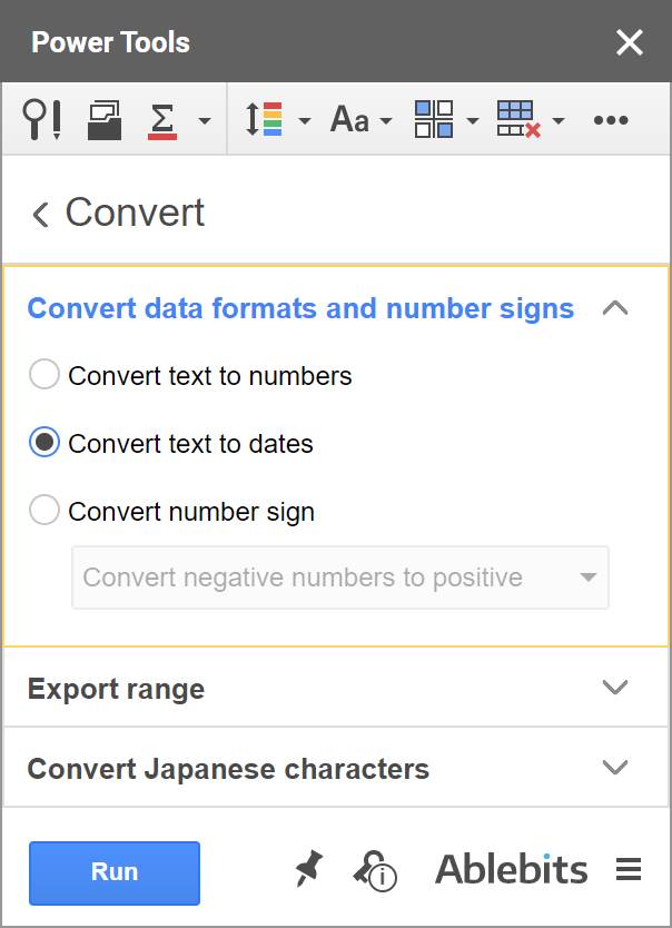
The tool recognizes all these custom formats in your Google Sheets and converts text to date so all cells become consistent and can be used for further reference:
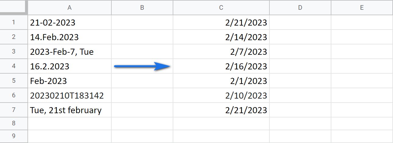
This is it! I hope by now you know how to change date format in Google Sheets and convert dates to numbers or text. Feel free to share other cool ways in the comments section below. ;)
 by
by
204 comments
I'm trying to get Google Sheets to calculate the duration (in hours and minutes) between a start date/time and an end date/time but I keep getting an error saying that it's recognizing my date/time inputs as text. I've tried custom formatting the date/time inputs so it registers, but I keep running into the same problem. I would like to keep the date/time inputs as YY/MM/DD - HHMM but can't seem to find a way to make it not register as a text for the calculation of the duration. Any help would be appreciated, thank you.
When you try to change the format with some cells in this 4/5/16 format they do not change while others do change to the 4/5/2016 format and I have dates in both formats, why does that happen?
Hello Sergio,
looks like Google Sheets doesn't read 4/5/16 as a date from the beginning. Try to apply a custom date format to this cell first (d/m/yy) before changing it to another required date format.
I have a sheet that receives data mapped directly from a web form. The date/time format of the form is dd/mm/yyyy hh:mm:ss. I want to format the date and remove the time but Google always interprets the first date number as the month. I changed the locale to UK, but it still recognizes the dd as mm, so when I try to change the date format to dd-MMM-yyyy, 08/05/2024 becomes 5 Aug 2024 instead of 8 May 2024. What can I do?
Hello SJ Thomas,
For me to be able to help you, I need to look at your spreadsheet. How you import the data, the formats applied - everything matters. Please share it (or its editable copy) with us (support@apps4gs.com) and specify where the dates are.
Note. We keep that Google account for file sharing only and don't monitor its Inbox. Do not email there. Once you share the file, just confirm by replying to this comment.
I'll look into it and try to help.
How do I convert date format mo/dd/yyyy so leading zeros show? For example... I want to convert 2/7/2023 to 02/07/2023. Some of my cells show leading zeros but I cannot seem to duplicate that fomatting for rest of the cells.
Hello Daniel,
Apply a custom format to your dates as described here. Each date unit offers an option to include a leading zero in the format.
Hi Natalia, I have a sheet that in a column, formatted as date time, presents some values in the format year/month/day hours:minutes:seconds other day/month/year hours:minutes:seconds and I can't convert everything into a single format (yyy-mm-dd hh:mm:ss) with none of the methods you explained above...
Can you help me?
Thank you
Enzo
Hi Enzo,
I'm sorry but your task is not clear. Please describe it in detail specifying some records you already have and how you want them to actually look.
Hi! So I am new to using Google Sheets. I am a Microsoft Excel user and would consider myself a bit better than a novice. I have been able to figure out how to set up a date formula in Excel that does not require me to type a forward slash but always displays it with one. I cannot seem to figure out how to do that in Google Sheets. I have the selected column cells set with custom date of mm/dd/yyyy, but when I type 02041999 it is only displaying as regular numbers, not as 02/04/1999. How do I fix that because I simply do not want to have to type the forward slash every time.
Thanks in advance for your replies!
Hi Susan,
In Google Sheets, it's impossible to make it treat numbers without separators (like slashes or dashes) as a date. In your case, I'd advise using a helper column with a formula that will turn your numeric string into a date:
=DATE(RIGHT(A1, 4), LEFT(A1, 2), MID(A1, 3, 2))
Just make sure you enter numbers with an apostrophe at the beginning: '02041999
And format the column with formulas as a date.
When I use a date in a cell with a function like adding two columns into one column I get integral numbers not the standard did-mm-yyyy
=TO_DATE(45388)
This converts the integral number to the correct date format 4/6/2024
Is there any other basic solution here.
Hello Deano,
Have you tried simply changing the format of the resulting cell?
Dear
I defined a new time format to be able to calculate the differences between times (mm:ss.00) but I can't apply to a selection of cells.
I can do it but if I look in the menu it's not chosen as format and my formula (difference in duration between 2 times) doesn't work because the cell contains text it says... Can someone help?
Hello Jana Vanden,
For me to be able to help you, please specify the exact formula you're using to calculate the time difference and the time format you're trying to apply.
I've got a csv file with the dates in mm/dd/yyyy format, and when I import it into my (UK region) Sheet it comes out as the same format, even when I do a Format>Number>Date on the column. I can do a regex transform, but is there a simple way of getting the dates to display in UK format?
Hi! Usually, when you import dates from a CSV file, they are written as text. To change the format, you need to convert the text to a date. You may find these instructions useful: DATEVALUE function for Google Sheets. Here's the easiest solution for your Google Sheets: convert text to dates using the Power Tools add-on.
I'm using scripts (getValues and setValues) to copy values (including dates) to an external document.
I noticed my document timestamp was incorrect, so I changed my document settings to the correct timezone.
Ever since then my scripts are adjusting the date before copying it, and all the transferred dates are out by 1.
How can I fix this?
Hello Marné,
We're always ready to help you, but we do not cover the programming area (script-related questions). You may try to find a solution here – an overview of Google Apps Script with a lot of helpful content and links:
https://developers.google.com/apps-script/overview
I hope you’ll find this information helpful. Sorry I can't assist you better.
Hi All,
How to Display Days or Month in Capital letters, like - MON, TUE, JAN, DEc etc. Thanks
Hi WizIT,
If you mean the date format, I'm afraid you can only use the existing writing. But if it's text, you can just change the case.
saya punya masalah dengan formula TEXT untuk seluruh Kolom A:A, dimana kolom yang kosong ikut dikonfersi menjadi text. berikut formula saya =TEXT(A:A;"dd mmmm yyyy"). saya ingin kolom yang kosong pada kolom A tidak ikut berubah menjadi TEXT
Hello Rolan,
I'm sorry, we provide assistance in English only. The TEXT function affects only the column where you put it. It doesn't format the data directly in your referred column A. So you can just select column A and apply the desired format from the Google Sheets menu.
Hi Natalia,
I've been through all your excellent and well explained responses, but don't seem to be able to find an answer to my query...
I get my bank statement online, and copy and paste the raw info into my own personal spreadsheet by greying everything out via the mouse, and use that for my own-designed accounts package! I've used this system for ten years, and while it isn't rocket science, I like to know what's happening and feel a bit happier if things are going well - or not!
The date of each transaction appears in one cell, with the shortened date format, i.e. 06 May 2023, and in the same cell, the recipient of the money I've sent is printed directly underneath the date, so I have a 'two tier' cell, which I cannot see how to split up! I have to do this manually, and sometimes run out of time as the bank logs me off pretty quickly!
I've tried all manner of functions, but never get anywhere near a result! I can do a regexreplace function on another cell, where the amount and the text is in the same plane, but the double-tier issue doesn't seem to work the same way!
Is it at all possible for me to separate the date from the recipient, and just have them in two adjoining cells to suit my accounts programme please?
With best wishes,
Mike A.
Hi Michael,
If I understand your task correctly and you need to split the data in a cell, I'd recommend using one of the methods from this blog post.
Hi Natalia,
That's great - thank you so much for such a swift response!
Best wishes,
Mike.
My pleasure, Mike!
Brilliant
The solution to change the date format using the QUERY function is the simplest I've seen. Great work. Thank you for solving this issue.
=QUERY(A1:C7,"select * format B 'd-mmm-yy (ddd)'")
You're most welcome, Jorge :) Appreciate your feedback!
Hi I have a big issue. I am trying to automate my work tasks and I have an account in google sheets which is linked to my Calendly and it downloads all the data from calendly into different collumns on my google sheets. One of them is the time. The cell with the time and date expresses the date in this form"07:00pm - Wednesday, April 5, 2023". I wanted to created an specific number for each one as sometimes i get interviews in my agenda from different days and i wanted the dates to be ordered from monday to friday each day with the correct hours. I had managed to do that with this formula
"=FECHANUMERO(DERECHA(B20;LARGO(B20)-ENCONTRAR(",";B20)-1)) + HORANUMERO(IZQUIERDA(B20;5))"
But today, it collapsed and I dont know why.
I wanted to know if there is a way in which I can again make it work or use a similar formula.
i will show how it used to look:
NUMBER VALUE TIME from calendly
45019,20833 05:00pm - Monday, April 3, 2023
45019,22222 05:20pm - Monday, April 3, 2023
45019,23611 05:40pm - Monday, April 3, 2023
45019,25 06:00pm - Monday, April 3, 2023
45019,26389 06:20pm - Monday, April 3, 2023
45019,27778 06:40pm - Monday, April 3, 2023
and now i have a message of error that says "El parámetro "April 5, 2023 " de DATEVALUE no se puede analizar como fecha/hora."
Hello Agustina,
For me to be able to help you better, please specify how the records look when Calendly returns them and how you need them to look as a result.
Is there a region that uses both $ and the ISO standard date format? I'm getting tired of constantly converting dates to YYYY-MM-DD, but the only work around I could find was setting my region to an area that does not use dollars.
Hello Rosalie,
Sorry, I can't say for sure as I don't have experience with all locales. However, you can apply the required date or custom currency format once, and then quickly copy/apply it using the standard Paint format tool: https://support.google.com/docs/answer/161768?co=GENIE.Platform%3DDesktop&hl=en#zippy=%2Ccopy-text-formatting-paint-format
Hi Natalia, I was reading your post but unfortunately my problem is more in the hour section which you kind of overlooked. I know, it must be the least used part of the date info but in my case is exactly, and only, what I need. I don't know if this goes beyond your expertice but I'm building a time sheet to calculate my worked hours in order to speed up my montly report. I found that manually entering the data is not only tedious but also prone to errors that could affect my paycheck. So I found a tutorial to convert 3 digit and 4 digit numbers into time using a Google Apps Script. It's working in converting my numbers into time format on the fly but it's not doing it correctly. When I enter "930" it converts it to "12:30", if i enter "830" it gives me "00:50". I tried changing the Locale in settings but it still converts it wrong. Can you guide into whatever might be happening here? Assuming there's nothing wrong in the script of course but in Google Sheets. Also, i'd like to know if after I make it to convert to time correctly I could simply create a formula to substract my Clock-in Time from my Clock-out Time and have the exact total of worked hours. I did it in a basic spreadsheet with no script applied and it seemed to work but it always gave weird time like, if I entered: 9:30 as clock-in time and 7:30 as clock-out time it gave me 10 hours total but it'd say "10:00 PM". It's funny it gets the total right when also assumes weird time inputs. Like 9:30 am as clock-in and 7:30 also am as clock out.
Hi Sergio,
I'm sorry but we don't cover the programming area (script-related questions). If the script converts time, I'd look for the problems there.
To add or subtract different time units, please see this blog post. It also covers cases like when you need to calculate more than 24 hours.
Also, if you just enter 9:30 and 7:30 and don't specify the part of the day (AM/PM), Google Sheets will automatically mark them as AM (select each cell and look at the formula bar, you'll see how Google Sheets understands the values). Hence, the result is 22:00, or 10:00 PM with the Time format.
Hello Natalia,
Under "How Google Sheets Formats dates" there's a couple of examples of how time is kept as an integer.
It's written that, 43,679.813 is August 2, 2019, 7:30PM.
Shouldn't the integer for 7:30 PM be .73 instead of .813?
Example:
31,528.058 is April 26, 1986, 1:23 AM
43,679.813 is August 2, 2019, 7:30 PM
Hello Marques,
You can check this by entering 7:30 PM into a cell and applying the Automatic format to it. You'll see 0.813
Thank you Natalia!
My pleasure :)
In cell in "Date is vaild" format is dd/mm/yyyy. How to change is yyyy-mm-dd in plain text ?
" Is valid date"
Hello Nontakorn,
I'm sorry, your question isn't clear. Could you elaborate, please? Thank you!
In cell function data validation " Is valid date " when i choose date. The format is dd/mm/yyyy but i want to format yyyy-mm-dd in plain text not use Format "Date" in toolbar. i want a plain text date is yyyy-mm-dd. Thanks><
Thank you for replying, Nontakorn.
What happens if you simply apply the required format (Format > Number > Plain text) to a cell with that data validation rule? It works for me. Though you will most likely have to re-enter the date in the required format.
Or use the formula from this part of the article to set the format.
Thank you
Hi Natalia!
I have a problem with the way google sheets interprets the dates I'm writting. I have a column for dates with the format dd-mm-yyyy. However, when I type a date such as 12-2-23 it assumes the date 23-12-2012 by default! What can I do? Thanks!
Hi Leonor,
I'd check the locale of the spreadsheet first. More about it and why it's important in this part of the article.
Then select your entire column (not just cells with the data) and apply the desired date format manually once more.