Though word and character count in Google Sheets are used in rare cases, it is still the functionality that some of us expect to see right in the menu. But unlike Google Docs, for Google Sheets, it is the LEN function that does that.
Even though there are many different ways to count characters in spreadsheets, today's blog post will cover the LEN function as its main purpose in tables is to – well, count :) However, it is hardly ever used on its own. Below you will learn how to use Google Sheets LEN correctly and find the most wanted formulas to compute characters in spreadsheets.
Google Sheets LEN function – usage and syntax
The main and the only purpose of the LEN function in Google Sheets is getting the string length. It is so simple that it even requires only 1 argument:
- it can take either the text itself in double-quotes:
=LEN("Yggdrasil") - or a reference to a cell with the text of interest:
=LEN(A2)
Let's see if there are any peculiarities in using the function in spreadsheets.
Character count in Google Sheets
I'll start with the simplest operation: do a character count in Google Sheets the most common way – by referencing a cell with the text using the LEN function.
I enter the formula to B2 and copy it down the entire column to count characters in each row:
=LEN(A2)
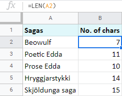
Note. The LEN function computes all characters: letters, numbers, spaces, punctuation marks, etc.
You may think that in a similar manner you could do a character count for the entire range of cells, like this: LEN(A2:A6). But, as bizarre as it is, it doesn't simply work this way.
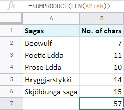
To total characters in several cells, you should wrap your LEN in SUMPRODUCT – the function that tallies up the numbers from entered ranges. In my case, the range is returned by the LEN function:
=SUMPRODUCT(LEN(A2:A6))
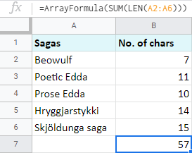
Of course, you could incorporate the SUM function instead. But SUM in Google Sheets doesn't process arrays from other functions. To make it work, you will have to add another function – ArrayFormula:
=ArrayFormula(SUM(LEN(A2:A6)))
How to count characters without spaces in Google Sheets
As I noted above, Google Sheets LEN function counts each and every character it sees including spaces.
But what if there are extra spaces added by mistake and you don't want to consider them for the result?
For cases like this, there's the TRIM function in Google Sheets. It checks the text for leading, trailing, and repeated spaces in-between. When TRIM is paired with LEN, the latter doesn't count all those odd spaces.
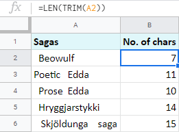
Here's an example. I added spaces in different positions in column A. As you can see, when on its own, Google Sheets LEN counts them all:
=LEN(A2)
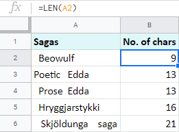
But as soon as you integrate TRIM, all extra spaces are ignored:
=LEN(TRIM(A2))
You can go further and make your formula disregard even those single spaces between words. The SUBSTITUTE function will assist. Though its main purpose is to replace one character with another, there's a trick to make it reduce spaces completely:
- text_to_search is the range you work with: column A, or A2 to be exact.
- search_for should be a space character in double-quotes: " "
- replace_with should contain empty double-quotes. If you're going to ignore spaces, you need to replace them with literally nothing (empty string): ""
- occurence_number is normally used to specify the instance to replace. But since I'm describing how to count characters without all spaces, I suggest you omit this argument as it is optional.
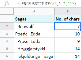
Now try and assemble all these into Google Sheets LEN and you'll see that no space is taken into account:
=LEN(SUBSTITUTE(A2, " ", ""))
Google Sheets: count specific characters
The same tandem of Google Sheets LEN and SUBSTITUTE is used whenever you need to count specific characters, letters, or numbers.
In my examples, I'm going to find out the number of occurrences for the letter 's'. And this time, I'll start with a ready-made formula:
=LEN(A2)-LEN(SUBSTITUTE(A2, "s", ""))
Let's break it down to pieces to understand how it works:
- SUBSTITUTE(A2, "s", "") looks for the letter 's' in A2 and replaces all occurrences with "nothing", or empty string ("").
- LEN(SUBSTITUTE(A2, "s", "") works out the number of all characters but 's' in A2.
- LEN(A2) counts all characters in A2.
- Finally, you subtract one from the other.
The result difference shows how many 's' there are in the cell:
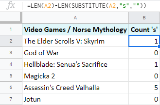
Note. You may wonder why B1 says there's only 1 's' in A2 while you can see 3?
The thing is, the SUBSTITUTE function is case-sensitive. I asked it to take all instances of 's' in lowercase and so it did.
To make it ignore text case and process letters in both lower and upper cases, you will have to call one more Google Sheets function for help: LOWER.
Tip. See other ways that change the text case in Google Sheets.
It is as simple as Google Sheets LEN and TRIM because all it requires is the text:
=LOWER(text)
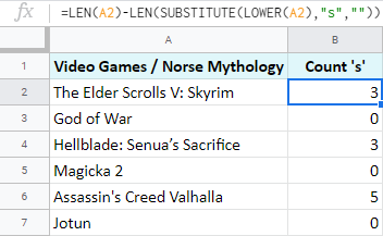
And all it does is turn the entire text string into lower case. This trick is exactly what you need to make Google Sheets count specific characters no matter their text case:
=LEN(A2)-LEN(SUBSTITUTE(LOWER(A2), "s", ""))
Tip. And as before, to count the total of specific characters in the range, wrap your LEN in SUMPRODUCT:
=SUMPRODUCT(LEN(A2:A7)-LEN(SUBSTITUTE(LOWER(A2:A7), "s", "")))
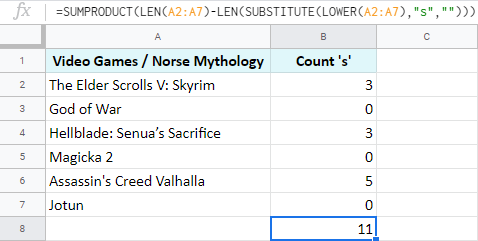
Count words in Google Sheets
When there are multiple words in cells, chances are you will need to have their number instead of the Google Sheets string length.
And though there are multiple ways of doing so, today I will mention how Google Sheets LEN does the job.
Remember the formula I used to count specific characters in Google Sheets? In fact, it will come in handy here as well. Because I'm not going to literally count words. Instead, I will count the number of spaces between the words and then simply add 1. Have a look:
=LEN(A2)-LEN(SUBSTITUTE((A2), " ", ""))+1
- LEN(A2) counts the number of all chars in the cell.
- LEN(SUBSTITUTE((A2)," ","")) removes all spaces from the text string and counts remaining chars.
- Then you subtract one from the other, and the difference you get is the number of spaces in the cell.
- Since words always outnumber spaces in a sentence by one, you add 1 at the end.
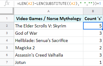
Google Sheets: count specific words
Finally, I'd like to share a Google Sheets formula that you can use to count specific words.
Here I have The Mock Turtle's Song from Alice's Adventures in Wonderland:
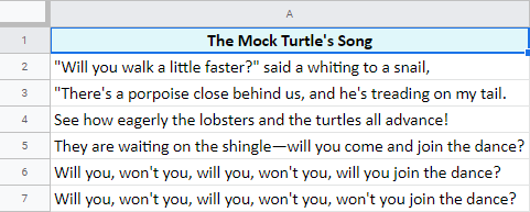
I want to know how many times the word 'will' appears in each row. I believe you won't be surprised if I tell you that the formula I need consists of the same functions as before: Google Sheets LEN, SUBSTITUTE, and LOWER:
=(LEN(A2)-LEN(SUBSTITUTE(LOWER(A2), "will", "")))/LEN("will")
The formula may look scary but I can assure you that it's easy to comprehend, so bear with me :)
- Since the text case doesn't matter to me, I use LOWER(A2) to turn everything to lowercase.
- Then goes SUBSTITUTE(LOWER(A2), "will",""))) – it gets rid of all occurrences of 'will' by replacing them with empty strings ("").
- After that, I subtract the number of characters without the word 'will' from the total string length. The number I get counts all characters in all occurrences of 'will' in each row.
Thus, if 'will' appears once, the number is 4 as there are 4 letters in the word. If it appears twice, the number is 8, and so on.
- Finally, I divide this number by the length of the single word 'will'.
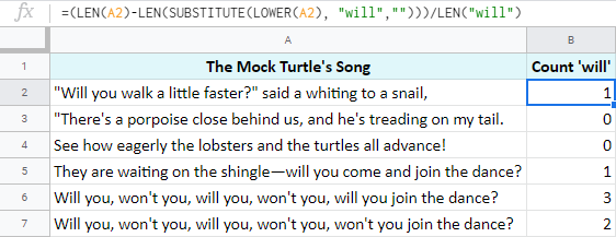
Tip. And again, if you'd rather get the total number of all appearances of the word 'will', just enclose the entire formula by SUMPRODUCT:
=SUMPRODUCT((LEN(A2:A7)-LEN(SUBSTITUTE(LOWER(A2:A7), "will", "")))/LEN("will"))
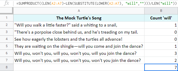
As you can see, all these cases of character-count are solved by the same patterns of the same functions for Google Sheets: LEN, SUBSTITUTE, LOWER, and SUMPRODUCT.
If some formulas still confuse you, or if you're not sure how to apply everything to your particular task, don't be shy and ask away in the comments section below!
 by
by
27 comments
Which formula would you use to count the number of sentences that contain a certain word or words.
For example: "I ran to the store to buy milk. It was on sale." This string has 1 sentence that contains the word "store" or "milk".
Hello Kelvin,
You can try a formula like this:
=ARRAYFORMULA(SUM(IF(REGEXMATCH(SPLIT(A2:A10, "."), "store|milk"), 1, 0)))
Replace A2:A10 with your range and store|milk with the required words.
Hi, I retype since I just notice the website displayed differently what I had input. So please ignore the first message.
I have a column D named Funding. It is a link to original column where it drag all of the funding for 1 location. I want to count how many funding a location receive. I face with issue that the funding is input with number value, from 0 to many. So when I count the fund, the system count the 0 as well, and return 1 for 0 funding.
Columns: C, D. E
Name: County, Funding, How many funding?
Columbia County gets No funding, but when I count, I use countif, it returns 1 as displayed in column: Columbia County; 0; 1
Morgan County gets 2 funding 18000 and 56000, I use countif, it returns with 2 fundings as I expect (display in column Morgan County; 18000, 56000; 2)
Can you please help me to make it return 0 instead of 1 for Columbia County
Thank you so much,
Hi Lokine,
If you work in Google Sheets, for me to be able to help you, please consider sharing an editable copy of your spreadsheet along with your COUNTIF formula with us: support@apps4gs.com. If you have confidential information there, you can replace it with some irrelevant data, just keep the format.
Please include the example of the result you'd like to get.
Note. We keep that Google account for file sharing only and don't monitor its Inbox. Please do not email there. Once you share the file, just confirm by replying to this comment.
I'll look into it and try to help.
In the meantime, feel free to check out this tutorial for the COUNTIF function in Google Sheets.
Yet, if you work in Excel, you need to post your question under this article.
Hi Natalia,
Thank you so much for quick reply.
I already sent the editable copy of the spreadsheet. I also tried the countif but it does not work in this case.
Thank you so much
Hi Lokine,
Thank you, I've got the file.
The thing is, you used LEN along with COUNTIF. LEN counts the number of characters in a cell, and you always added 1 on top of that, hence, you didn't get 0 as you needed. Use this formula instead (it's for D2 but you can adjust it for other cells):
=IF(C2=0,0,COUNTIF(SPLIT(C2,","),">0"))
Hi Natalie,
Thank you so much for your help. Yesssssss, it works! You guys are so amazing!
All the best!
Happy to help, Lokine! :)
What's the formula to find which is the most frequent character in a cell in Google Sheets?
Hello Jo,
Try this formula:
=ArrayFormula(CHAR(MODE(CODE(MID(A2,ROW(INDIRECT("1:"&LEN(A2))),1)))))
Hello. I parsed text in a text document into multiple rows of 1 word tags. I then converted that to a CSV file, and uploaded to Google Sheets. I now want to take that google sheet - a single row of 1 word tags, plus some other rows with 3 or 4 miscl. words that will prove to be not significant in number, and count the number of cells in a column that have the value of "APPLES", as well as the count for how many with the value of "ORANGES". Is there an easier way to do this, then LEN? Whatever the simplest way to do it is, can you show me an example? Thanks.
Hello Chris,
to count the number of cells based on the condition, you need to use the COUNTIF function.
But if this doesn't really suit your task, please describe it in detail. Feel free to share your sample data with us (support@apps4gs.com). Please include the result you expect to get and shorten the tables to 10-20 rows.
Note. We keep that Google account for file sharing only and don't monitor its Inbox. Please do not email there. Once you share the file, just confirm by replying to this comment.
I'll look into your task and try to help.
Hi, thank you for the detailed article.
I'm actually having trouble trying to apply the word count formula to multiple columns (about 20 consecutive columns) that include alphanumerics including dates like 22/02/2022 or February 22, 2022. I've tried the below formula but it doesn't work for numbers:
=sum(arrayformula(len(regexreplace(regexreplace(R8:AP8,"\S+","a"),"\s",""))))
Please help me out, I'd be grateful!
Hi Vrunek,
For me to be able to help you, please share a small sample spreadsheet with us (support@apps4gs.com) with 2 sheets: (1) a copy of your source data (2) the result you expect to get (the result sheet is of great importance and often gives us a better understanding than any text description). I kindly ask you to shorten the tables to 10-20 rows.
Note. We keep that Google account for file sharing only and don't monitor its Inbox. Please do not email there. Once you share the file, just confirm by replying to this comment.
I'll look into your task.
HI Natalia,
I've shared the requested spreadsheet. Please do have a look and let me know. Thank you!
Hi Vrunek,
Thank you for the spreadsheet. Please see the Result sheet, I added formulas there:
=SUM(G2,COUNTA(SPLIT(TEXTJOIN(" ", true, R2:AP2), " ")))
Hi Natalia,
Thank you so much for this, this works perfectly for me. Really grateful to the Ablebits Team for helping me out. Will surely recommend your products to my associates. Thanks again! :)
You're most welcome, Vrunek, glad I could help! :)
=SUM(LEN(M2:U2)) I have this formula on excel but need to do the same thing on google sheets. What would be the formula for google sheets?
Hello Ro,
Try this one:
=SUM(Arrayformula(LEN(M2:U2)))
Feel free to learn more about the ArrayFormula function in this blog post.
So I run a high ranking guild in a video game and keep track of everyone's attacks, draws, and losses when we fight other guilds. We have so many attacks and I keep track of everything in the format 'w,d,L' etc. and I have the track record spread over multiple rows. For example, I am using this string '=SUMPRODUCT(LEN(J186:W186)-LEN(SUBSTITUTE(J186:W186, "w", "")))' to calculate totals over a row but need to add the total between multiple rows. How do I add 2 different rows together in this formula? I apologize if I'm not as clear as I'd like to be about this.
Essentially, I want to add that row with:
=SUMPRODUCT(LEN(B222:F222)-LEN(SUBSTITUTE(B222:F222, "w", "")))
Hello!
If I understand your task correctly, the following formula should work for you:
=SUM(LEN(B222:F222))-SUM(LEN(SUBSTITUTE(B222:F222, "w","",1)))
I hope my advice will help you solve your task.
Hello! This was an excellent post with formulas I hope to try. Here’s what I’m hoping it could be used for-can you assist me in knowing if it will work? I have to sift through a lot of online reviews/comments and provide analysis on “how many times a reviewer used certain words-like “happy”, “angry”, compassionate, etc. my hope is to use one of these words in the string of cells to easily identify the count. I’m doing something else which is quite tedious.. many thanks in advance for your kind assistance!
Hello Haley,
If I understand you correctly and you need to count the number of times a certain word appears, you should use the COUNTIF function. We have an entire blog post about it, please take a look:
Google Spreadsheet COUNTIF function with formula examples
Thanks for this great post!! Very clear and informative.
I have 1 question though...
=LEN(A2)-LEN(SUBSTITUTE(A2, "s", ""))
This formula is almost exactly what I need. Except, I dont want to count for "s", I want to count for the value in a specific cel (say C1, which will contain S). This is so I can easily change the S I am looking for into a different letter.
But I cannot seem to adjust the formula to make it count the text in a cell...
Curious to see if you have a solution.
Thanks in advance!
Sorry... solved it.... (forgot some brackets :S)
=LEN(A2)-LEN(SUBSTITUTE((A2);(C1);""))
Thank you for your feedback.
You don't actually need brackets for cell references. Instead, I'd recommend using dollar signs to make the reference absolute so it doesn't change when copied to other cells:
=LEN(A2)-LEN(SUBSTITUTE(A2;$C$1;""))