In my previous blog post, I described different means to find and process duplicates in your spreadsheet. But in order to spot them instantly, it would be best to highlight them with color.
And today I will try to cover the most popular cases for you. You will highlight duplicates in Google Sheets using not only conditional formatting (there are different formulas based on the spread of duplicates in your table) but also a special add-on.
Highlight duplicate cells in a single Google Sheets column
Let's start with the basic example. It is when you have just one column with repeated values:

Tip. I'm going to use conditional formatting in every but the last case today. If you're not familiar with it, get to know it in this blog post.
Here's how to highlight duplicate cells in one Google Sheets column:
- Go to Format > Conditional formatting in the Google Sheets menu:

- You will see the Conditional format rules window with the Single color tab opened by default:

- Select the range of cells where you want to highlight dupes (in the apply to range field) — A2:A10 in my example:

- Under Format rules, pick Custom formula from the drop-down:

- And enter the following formula:
=COUNTIF($A$2:$A$10,$A2)>1Note. Formulas in conditional formatting are dynamic. Hence, in this COUNTIF, I lock only A in A2 with a dollar sign. This way, the formula will handle each cell from column A. You will learn more about this trick with cell references in this article. - Select any color from the Formatting style to highlight those duplicates.
- Click Done.
That COUNTIF formula will scan your column A and tell the rule which records appear more than once. All these duplicate cells will be colored according to your settings:

Tip. See how to count cells by color in Google Sheets in this article.
Highlight duplicates in multiple Google Sheets columns
It may happen that repeated values will be in more than one column:
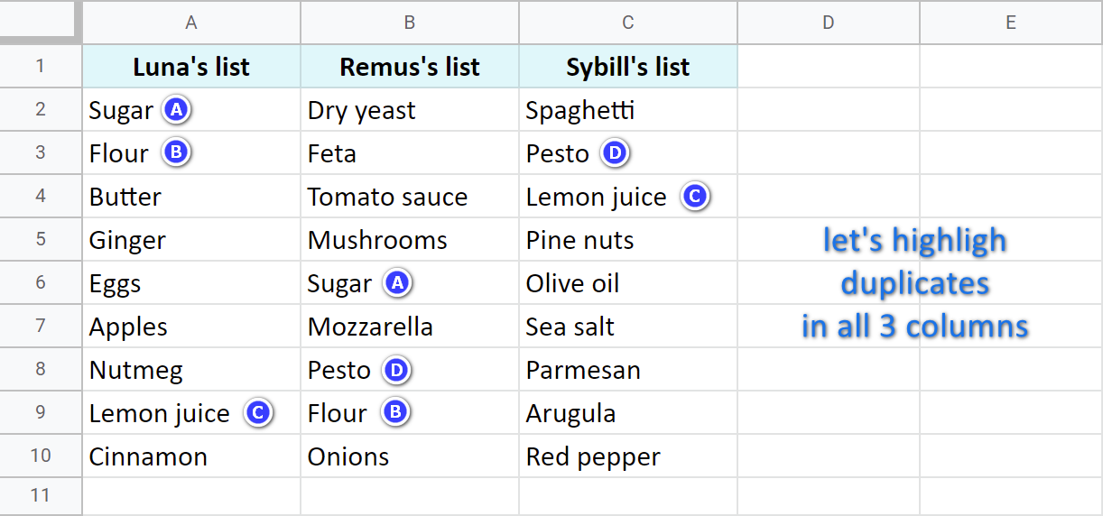
How do you scan and highlight duplicates in all 3 Google Sheets columns then? Using the conditional formatting as well. The drill is the same as above with a few slight adjustments:
- Select A2:C10 as a range to color repeated cells within
- Change the range for Custom formula as well:
=COUNTIF($A$2:$C$10,A2)>1
This time, remove the dollar sign from A2. This will let the formula count all occurrences of each cell from the table, not just from column A.Tip. Read this article to learn more about relative, absolute, & mixed cell references.
- Pick a color in the Formatting style section and hit Done

This COUNTIF scans all 3 columns and counts how many times each value appears in the whole range. If more than once, conditional formatting will highlight these duplicate cells in your Google Sheets table.
Highlight the entire row if duplicates are in one column
Next up is the case when your table contains different records in each column. But the entire row in this table is considered as a single entry, a single piece of information:
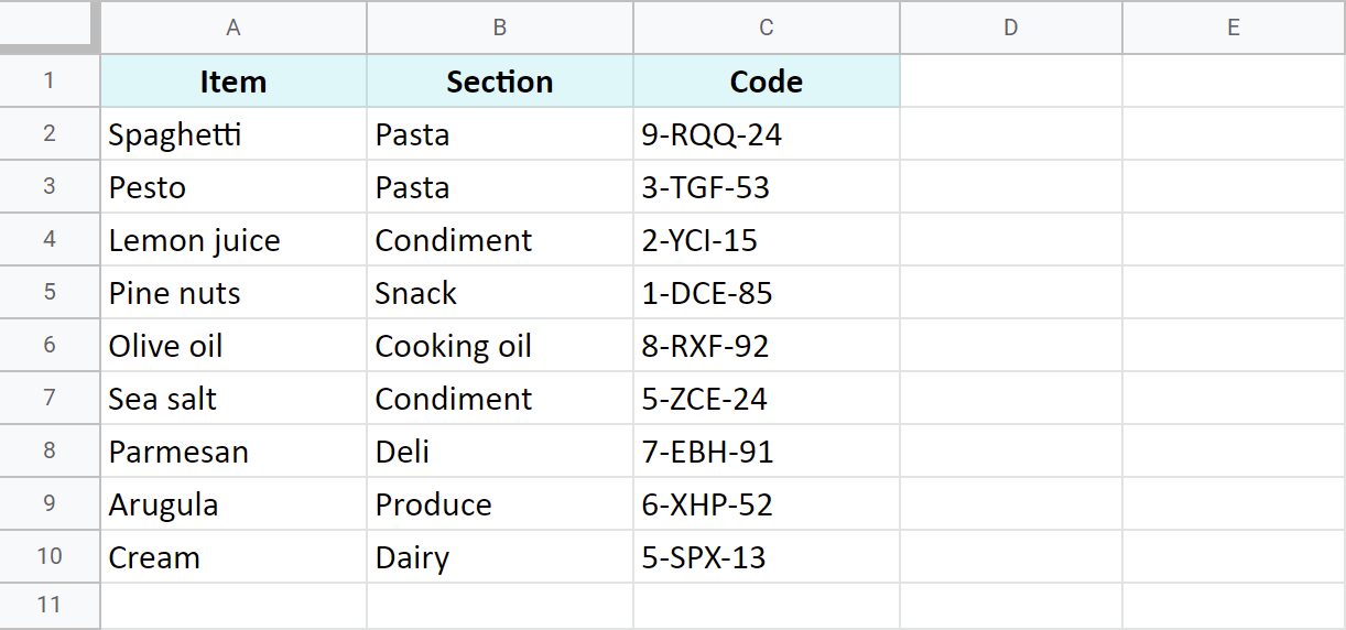
As you can see, there are duplicates in column B: pasta & condiment sections occur twice each.
In cases like this, you may want to treat these entire rows as duplicates. And you may need to highlight these duplicate rows in your Google spreadsheet altogether.
If that's exactly what you're here for, make sure to set these for your conditional formatting:
- Apply the rule to the range A2:C10
- And here's the formula:
=COUNTIF($B$2:$B$10,$B2)>1
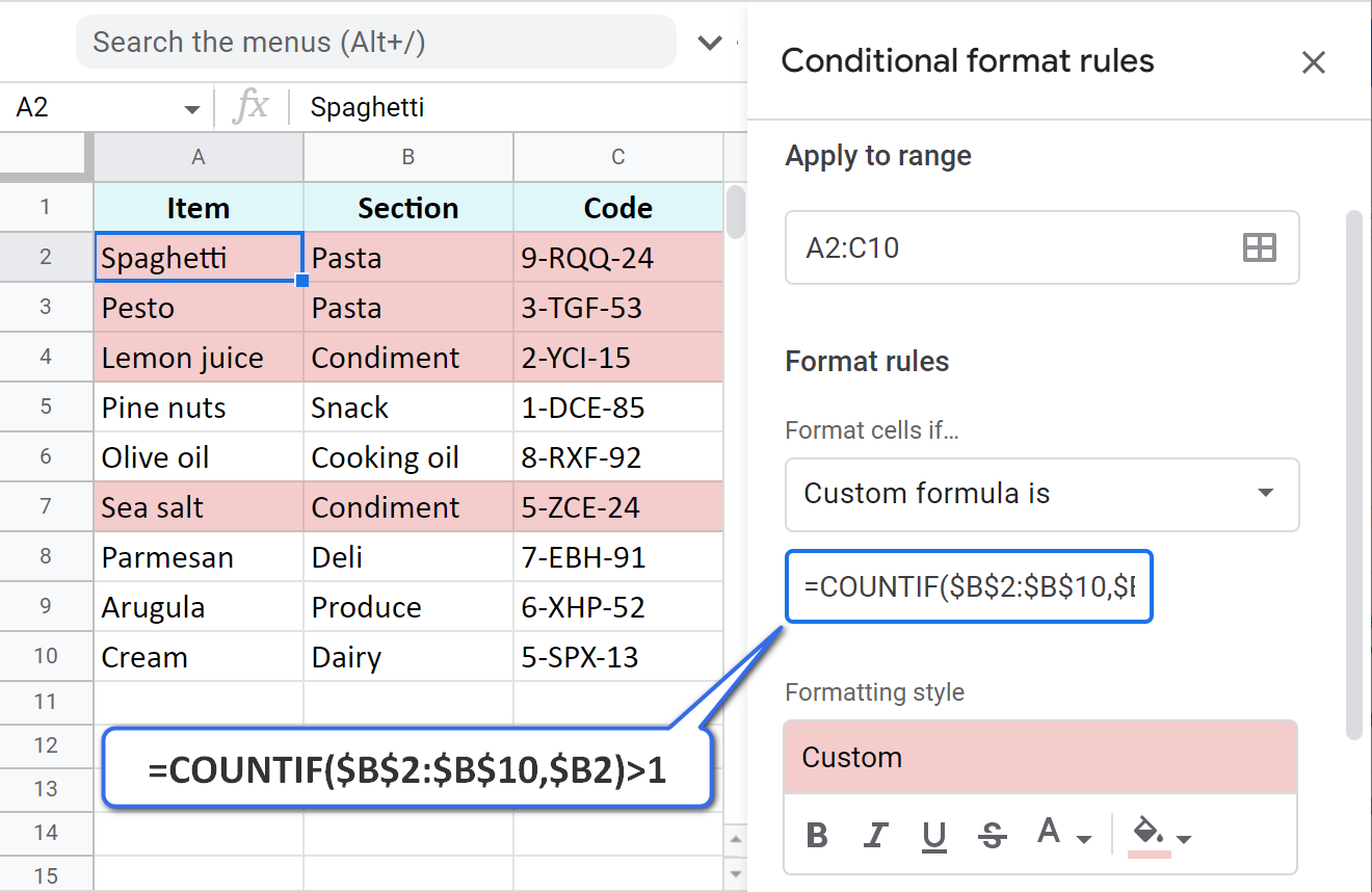
This COUNTIF counts records from column B, well, in column B :) And then the conditional formatting rule highlights not just duplicates in column B, but the related records in other columns as well.
Highlight complete row duplicates in spreadsheets
Now, what if the entire row (with the same records in all columns) appears several times in your table?
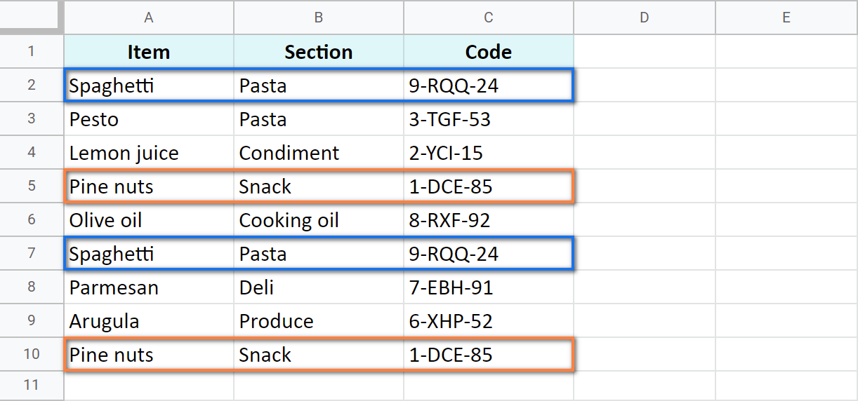
How do you check all 3 columns through the table and highlight absolute duplicate rows in your Google sheet?
Using this formula in conditional formatting:
=COUNTIF(ArrayFormula($A$2:$A$10&$B$2:$B$10&$C$2:$C$10),$A2&$B2&$C2)>1

Let's break it down into pieces to understand how it works:
- ArrayFormula($A$2:$A$10&$B$2:$B$10&$C$2:$C$10) concatenates every 3 cells from each row into one text string that looks like this: SpaghettiPasta9-RQQ-24
Thus, in my example, there are 9 such strings — one per row.
- Then COUNTIFS takes each string (starting from the first one: $A2&$B2&$C2) and looks for it among those 9 strings.
- If there's more than one string (>1), these duplicates get highlighted.
Tip. You may learn more about COUNTIF and the concatenation in Google Sheets in the related articles.
Highlight actual duplicates — 2n, 3d, etc instances
Let's suppose you'd like to keep the 1st entries of duplicate rows intact and see all other occurrences if there are any.
With just one change in the formula, you'll be able to highlight these 'real' duplicate rows — not the first entries, but their 2nd, 3rd, 4th, etc instances.
So here's the formula I suggested right above for all duplicate rows:
=COUNTIF(ArrayFormula($A$2:$A$10&$B$2:$B$10&$C$2:$C$10),$A2&$B2&$C2)>1
And this is the formula you need to highlight only duplicate instances in Google Sheets:
=COUNTIF(ArrayFormula($A$2:$A2&$B$2:$B2&$C$2:$C2),$A2&$B2&$C2)>1

Can you see the difference in the formula?
It's in the first COUNTIF argument:
$A$2:$A2&$B$2:$B2&$C$2:$C2
Instead of mentioning all rows like in the first formula, I use only the first cell of each column.
It lets each row to look only above to see if there are the same rows. If so, every current row will be treated as another instance or, in other words, as an actual duplicate that will be colored.
Formula-free way to highlight duplicates — Remove Duplicates add-on for Google Sheets
It's not a secret that any formula and conditional formatting require a learning curve. If you're not ready to devote your time to those, here's the easiest solution.
Remove Duplicates add-on for Google Sheets will highlight duplicates for you.
It takes just a few clicks on 4 steps. There's a separate step for each action so you won't get confused:
- First, the add-on offers an intuitive way to select your data:

- Our add-on knows how to highlight not only duplicates but also uniques. And there's an option to ignore 1st instances as well — all on step 2:

- Next, you pick columns you'd like to check for duplicates:

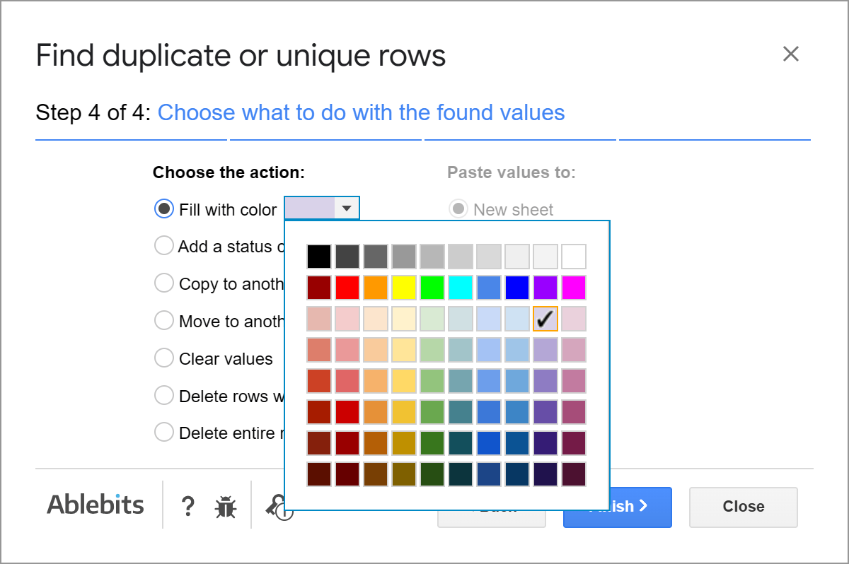
- And finally, the option to highlight found duplicates is just a radio button with a color palette on the last step:
Tip. Here's a video that shows the add-on in action. It may be a bit old since at the moment the add-on has more to offer, but it's still the same add-on:
Highlight duplicates on schedule using the add-on
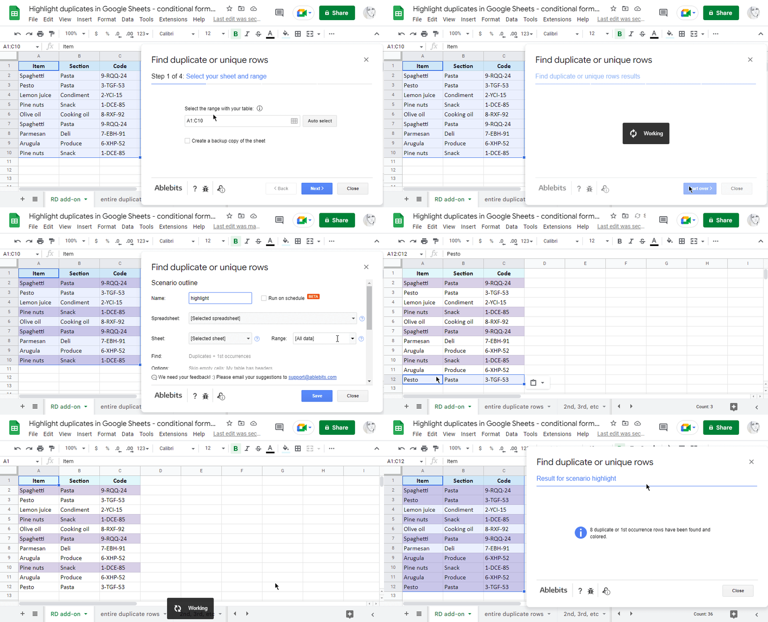
All the steps with their settings that you select in the add-on can be saved and reused in a click later or even scheduled to a certain time to autostart.
Here's a 2-minute demo video to back up my words (or see below for a couple animated images):
And here's a short animated image instead showing how to save and run scenarios once your data changes:
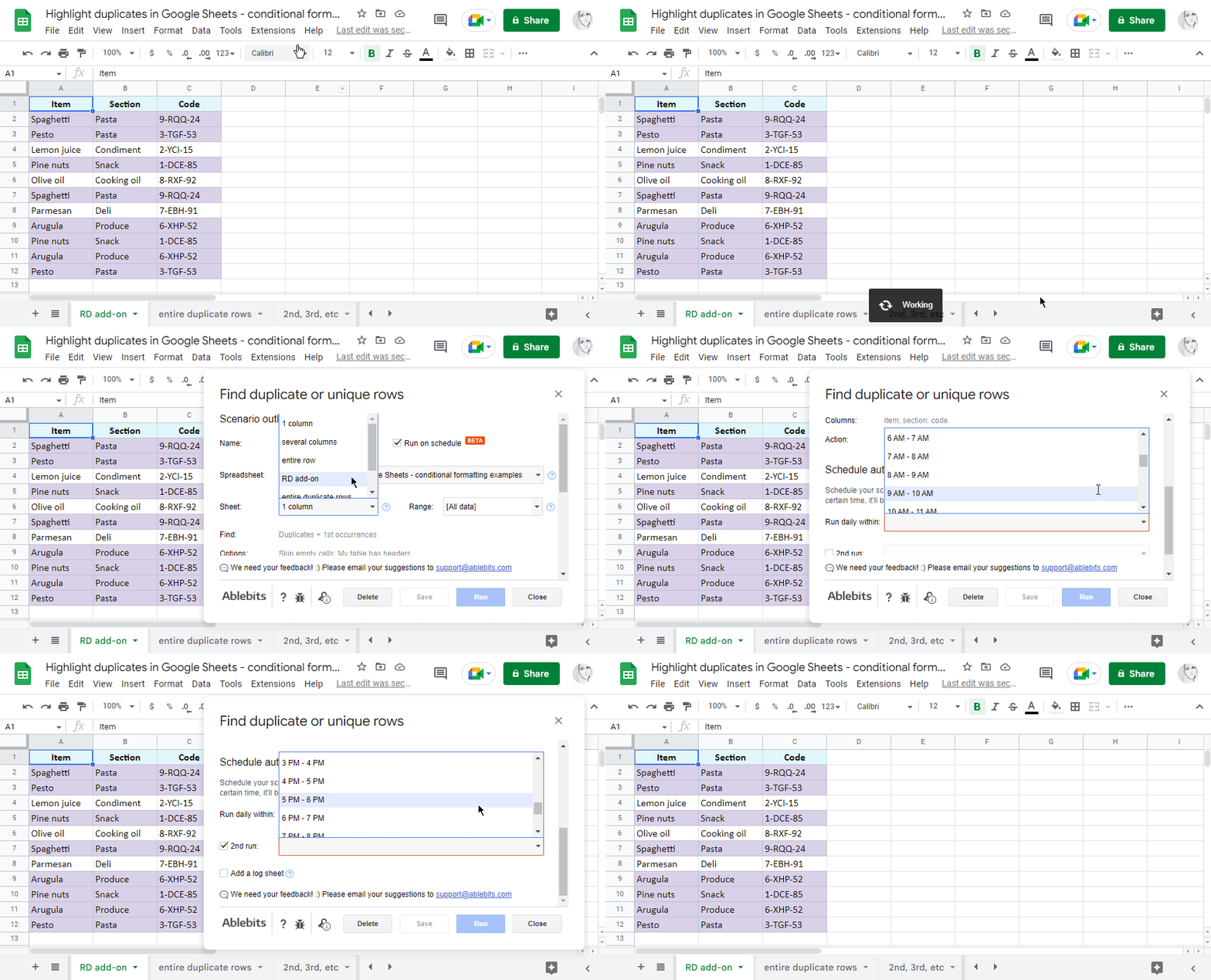
What's even better, you can schedule those scenarios to autostart a few times a day:
No worries, there's a special log sheet available for you to track all automatic runs & make sure they work correctly:

Just install Remove Duplicates from the Google Sheets store by clicking the button below.
As soon as you try it on your data, you'll see how much time and nerves it saves on getting those records colored correctly. Yes, without any formulas and in just in a few clicks ;)
Video: How to highlight duplicates in Google Sheets
This 1,5-minute video shows 3 quickest ways (with and without formulas) to find & highlight duplicates in Google Sheets. You will see how to color 1 column or entire rows based on duplicates, even automatically.
Practice spreadsheet
Highlight duplicates in Google Sheets - conditional formatting examples (make yourself a copy to practice)
 by
by
52 comments
=COUNTIF(ARRAYFORMULA($B$2:$B$10&$D$2:$D$10&$G$2:$G$10),$B2&$D2&G2)<1.
Why this farmula is not wokring?everything seems fine.
Waqar, your formula will always return FALSE because the criterion ($B2&$D2&G2) is part of the first row of the ARRAYFORMULA, since it’s included in the range, and the result of the COUNTIF will be at least 1.
Sorry, doesn't work.
Hello Enrique,
For me to be able to help you, please specify what exactly doesn't work and describe your problem/task in detail. Thank you.
Great guide on highlighting duplicates in Google Sheets! Your step-by-step approach makes it easy to follow, especially with the clear explanations of conditional formatting and formulas. I appreciate the tips on handling multiple columns too. This will definitely save time and enhance spreadsheet organization. Thanks for sharing these valuable techniques!
Thank you for your feedback!
Hi! Thank you for this!
I'm trying to highlight names over multiple tabs in the same Google worksheet, but the names are spread over 2 columns (Last Name, First Name). I can get it to highlight duplicates in the same sheet over two columns, or over two tabs with a single column, but I'm struggling putting the two together. The names start at A3 and B3 on both sheets.
=COUNTIFS($A:$A, $A3, $B:$B, $B3)>=2
This works for highlighting duplicate names over the 2 columns in the same tab/sheet.
=COUNTIF(INDIRECT("Sheet2!$A:$A"),A3)>0
This works to highlight just the last names from column A that appear in both sheets.
=COUNTIF(INDIRECT("Sheet2!$A:$B"),A3)>0
This highlights both names, but will also highlight just the first or last name if that repeats, which ends up with additional highlights I don't need. I want exact match over both columns.
I also tried to make a 3rd column with the names combined (then hid it) to get the duplicates that way, but it would only highlight the cells in column A, even though the applied range is A:B.
How can I combine these functions? Thank you in advance!
Hello Katrina,
Please read this article to learn how to compare two tables & highlight duplicate data between them.
Hi!
I've just sent a comment saying that the "Highlight duplicates in multiple Google Sheets columns" using =COUNTIF($A$2:$C$10,A2)>1 was not working for me then I managed to correct it.
In a table like:
| A | B | C |
1| | | |
2| | | |
3| | | |
I had to let the formula like this:
=COUNTIF($A:$C;A1)>1
This will high light each duplicated cell.
Also, my primary intention was to highlight only values duplicated in columns, but not rows. Then I managed to do that using:
=COUNTIF(A$1:A$40;A1)>1
Hi Georges,
It's good to know you managed to tweak the formula as needed! Thank you for sharing your solution with us :)
Hi!
At first, thank you for this amazing tutorial!
I was trying to apply the "Highlight duplicates in multiple Google Sheets columns" but it does not seem to be working.
I have an ABC table with 5 lines. I've place the conditional formar as:
Range: A1:C5
Formula: =COUNTIF($A$1:$C$5;A1)>1
It should set the cell color to green, but it doesnt.
My local is Brasil so ";" is correct. But I've already tried colon.
Of I place the formula in a cell, it will only show "TRUE" if the A1 cell has the duplicated data.
Do you have any idea of what could be the problem?
I've shared the link https://docs.google.com/spreadsheets/d/17S0Eo5x2I7LzAubw0pu0Z34Cvjzhx8vhnYfSDrrGkDs/edit#gid=0 with for support@apps4gs.com if you want to check.
Thanks in advance for any help.
...My local is Brasil so ";" is correct...
Thank you my Brazilian friend) The same here in Ukraine.
Hello dear,
Thanks for you tutorials ,
May you please help me with that, I need to find the duplicates depends on a specific date,
Hello Khairy,
Please describe your task in detail, I'll see if I can help.
Hello
The tutorial is great! Thank you for it!
I need duplicates from column E to be highlighted when the date matches today's date from column A.
I played with various formulas but every time I ran into the same problem: the formula would highlight values from column E if the row had today's date, but it was the only entry on today's exact date, the reason it was highlighted is that the same value in E column was repeated on previous dates.
The formula I'm currently using is:
=AND(COUNTIF(E:E,E1)>1,A1=TODAY())
Is there any way for the formula to ignore previous dates?
Thank you for your feedback, Victoria!
For me to be able to help you, please consider sharing an editable copy of your spreadsheet with us (support@apps4gs.com) including your conditional formatting rule and a sample of the expected result. I'll look into it.
Note. We keep that Google account for file sharing only and don't monitor its Inbox. Please do not email there. Once you share the file, reply to this comment. Thanks.
good post
Thank you, dede!
How can we use different color for different duplicate values
Hello Paras,
I'm afraid you won't be able to do that with one simple formula or so.
If you want to try without the script, here's an example for a short list of names in A2:A8. First, assign each unique name a number in column B with the following formula:
=IF(COUNTIF($A$2:A2, A2)=1, MAX($B$1:B1)+1, VLOOKUP(A2, $A$1:$B1, 2, FALSE))
Copy the formula down the column.
Then you need to create as many conditional formatting rules as there are unique names. For example, for a first 'name + number 1' the rule will be:
=AND(COUNTIF(ArrayFormula($A$2:$A2&$B$2:$B2&$C$2:$C2),$A2&$B2&$C2)>1,$B2=1)
For the next 'name + number 2' the rule will be:
=AND(COUNTIF(ArrayFormula($A$2:$A2&$B$2:$B2&$C$2:$C2),$A2&$B2&$C2)>1,$B2=2)
You change the number at the very end of the formula in each rule based on the number assigned to the name in column B.
If you'd rather avoid so many formulas, you may try to find a solution here – an overview of Google Apps Script with a lot of helpful content and links:
https://developers.google.com/apps-script/overview
Thank you, i found solution to find duplicates
How to delete entire raw if it has duplicate cell
Hello Sanjay,
You will find different ways of removing rows with duplicates in this article. This one is the quickest and doesn't require formulas.
Great post. Thanks for sharing this article.
Thank you for your feedback! Happy to know the article is useful :)
Yes this worked but highlighted one of the duplicate cells and another some other cell. Can you solve ?
Hello Sanket Saliyan,
I'm sorry, I don't understand what you mean. What method have you tried and what has gone wrong?
Hey there!
Thx for the awesome info!
Is it possible to have the "find duplicates" keep going as I fill in the cells?
Example:
I've already ran the check and no duplicates were found, however, I now add another cell within the range that IS a duplicate, can it immediately fill in the cell with a certain color?
Or the only way is to run the formula AFTER all the cells are filled?
Thx a million! :)
Hey Nadav,
Thank you for your kind feedback :)
As for your question, if you mean the Remove Duplicates add-on described at the end, you need to run it each time after entering more records because there is no technical possibility to keep it constantly running in the background. But there are scenarios available that speed up the process: you run the add-on with just one click or even schedule its auto-start every hour or so.
If your question is about conditional formatting rules that you are to set up manually, you just need to indicate a bigger range in advance in the Apply to range field.
This worked for me (with a tiny bit of adjusting)...
But my Issue/question is:
Issue: Every duplicate is the same color... so if there is a string of duplicates in a row, it will highlight all of them (visually) as one group.
Question: is there a way to have alternating colors so that it's easier to tell when one group of duplicates stops, and another begins?
Hello Myers,
Sorry, it's impossible with one formula or setting. You'd need to create multiple conditional formatting rules and specify different colors for the exact values. Or use Google Apps Script to code something like this for your task.
Is it possible to exclude blanks for duplicates highlights in the same row? In other words, I no need the blank cells to be highlighted.
I have same issue with Raghavi .
i use this formula: =COUNTIF(ArrayFormula($I$3:$I$165&$J$3:$J$165),$I3&$J3)>1
It's highlight all the duplicate including the blank cells.
Thanks
Hello Durrah,
The same solution as Raghavi found will help you:
=AND(COUNTIF(ArrayFormula($I$3:$I$165&$J$3:$J$165),$I3&$J3)>1,$I3<>"")
Hi,
I'm getting almost, but the formula I'm using is highlighting the FIRST value, the original one, but I need to highlight the second or more duplicated value.
This is the formula I'm using:
=CONTAR.SI($B4:$B$5500,B)>1
=COUNTIF($B4:$B$5500,B)>1
What I need is to highlight the second repeated value.
Thanks in avance.
Hi ILIANA,
Please read this part to see how to highlight duplicate values keeping the original value intact.
I am using your conditional formatting formula in Google Sheets to "Highlight the entire row if duplicates are in one column": =COUNTIF($B$2:$B$10,$B2)>1
I have email addresses in column C, so I modified my formula to be: =COUNTIF($C$2:$C$100,$C2)>1
This highlights the incorrect rows, the first duplicate, and the row above it, but the second instance is below not above. Wish I could attach a screenshot but let's say I have a duplicate email in row 3 and 4. Conditional formatting highlights row 2 and 3. :(
Confusing! Any idea why this is?
Hi Loren,
Could you please check what you have in the Apply to range field?
This dosent work
Hello Akshay,
Which way didn't work for you exactly? Any details on what you tried and how your data is arranged would help me help you :)
Thank you
You're most welcome, Sangram!