 by
by When you need to find data in your sheet that corresponds to a certain key record, it is usually Google Sheets VLOOKUP you turn to. But there you go: VLOOKUP slaps you with limitations almost immediately. That's why you'd better increase the resources for the task by learning INDEX MATCH.
INDEX MATCH in Google Sheets is a combination of two functions: INDEX and MATCH. When used in tandem, they act as a better alternative for Google Sheets VLOOKUP. Let's find out their capabilities together in this blog post. But first, I'd like to give you a quick tour of their own roles in spreadsheets.
Google Sheets MATCH function
I'd like to start with Google Sheets MATCH because it's really simple. It scans your data for a specific value and returns its position:
- search_key is that record you're looking for. Required.
- range is either a row or a column to look in. Required.
Note. MATCH only accepts one-dimensional arrays: either row or column.
- search_type is optional and defines if the match should be exact or approximate. If omitted, it is 1 by default:
- 1 means the range is sorted in ascending order. The function gets the largest value less than or equal to your search_key.
- 0 will make the function look for the exact match in case your range is not sorted.
- -1 hints that records are ranked using descending sorting. In this case, the function gets the smallest value greater than or equal to your search_key.
Here's an example: to get a position of a certain berry in the list of all berries, I need the following MATCH formula in my Google Sheets:
=MATCH("Blueberry", B1:B10, 0)

Google Sheets INDEX function
While MATCH shows where to look for your value (its location in the range), Google Sheets INDEX function fetches the value itself based on its row and column offsets:
- reference is the range to look in. Required.
- row is the number of rows to offset from the very first cell of your range. Optional, 0 if omitted.
- column, just like row, is the number of offset columns. Also optional, also 0 if omitted.
If you specify both optional arguments (row and column), Google Sheets INDEX will return a record from a destination cell:
=INDEX(A1:C10, 7, 1)

Skip one of those arguments and the function will get you the entire row or column accordingly:
=INDEX(A1:C10, 7)

How to use INDEX MATCH in Google Sheets — formula examples
When INDEX and MATCH are used together in spreadsheets, they are at their mightiest. They can absolutely substitute Google Sheets VLOOKUP and fetch the required record from a table based on your key value.
Build your first INDEX MATCH formula for Google Sheets
Suppose you'd like to get the stock info on cranberry from the same table I used above. I only swapped columns B and C (you'll find out why a bit later).
- Now all berries are listed in column C. Google Sheets MATCH function will help you locate the exact row of the cranberry: 8
=MATCH("Cranberry", C1:C10, 0) - Put that whole MATCH formula to a row argument in the INDEX function:
=INDEX(A1:C10, MATCH("Cranberry", C1:C10, 0))This one will return the entire row with cranberry in it.
- But since all you need is the stock info, specify the number of the lookup column as well: 3
=INDEX(A1:C10, MATCH("Cranberry", C1:C10,0), 2) - Voila!
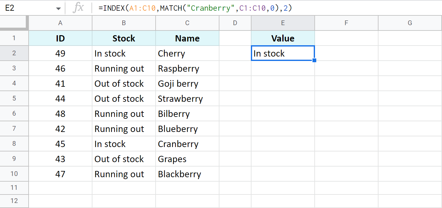
- You can go further and give up that last column indicator (2). You won't need it at all if you use only the lookup column (B1:B10) rather than the entire table (A1:C10) as the first argument:
=INDEX(B1:B10, MATCH("Cranberry", C1:C10, 0))


Tip. A more convenient way to check the availability of various berries would be to place them in a drop-down list (E2) and refer your MATCH function to the cell with that list:
=INDEX(B1:B10, MATCH(E2, C1:C10, 0))
Once you select the berry, the related value will change accordingly:

Why INDEX MATCH in Google Sheets is better than VLOOKUP
You already know that Google Sheets INDEX MATCH looks your value up in a table and returns another related record from the same row. And you know that Google Sheets VLOOKUP does exactly the same. So why bother?
The thing is, INDEX MATCH has some major advantages over VLOOKUP:
- Left-side lookup is possible. I changed the columns places earlier to illustrate this one: INDEX MATCH function in Google Sheets can and does look to the left of the search column. VLOOKUP always searches the very first column of the range and looks for matches to its right — else, it gets only #N/A errors:

- No messed up references when adding new columns and moving existing ones. If you add or move columns, INDEX MATCH will reflect the changes automatically without meddling in the result. Since you use column references, they are instantly adjusted by Google Sheets:

Go ahead and try to do this with VLOOKUP: it requires the order number rather than cell references for a lookup column. Thus, you'll just end up getting the wrong value because another column takes the same place — column 2 in my example:

- Considers text case when necessary (more on this right below).
- Can be used for vertical lookup based on multiple criteria.


I invite you to look at the last two points in detail below.
Case-sensitive v-lookup with INDEX MATCH in Google Sheets
INDEX MATCH is a go-to when it comes to case-sensitivity.
Supposing all berries are being sold in two ways — loose (weighed at the counter) and packed in boxes. Hence, there are two occurrences of each berry written in different cases in the list, each with its own ID that also vary in cases:

So how can you look up the stock info on a berry sold in a certain way? VLOOKUP will return the first name it finds no matter its case.
Luckily, INDEX MATCH for Google Sheets can do it correctly. You'll just need to use one additional function — FIND or EXACT.
Example 1. FIND for case-sensitive Vlookup
FIND is a case-sensitive function in Google Sheets which makes it great for case-sensitive vertical lookup:
=ArrayFormula(INDEX(B2:B19, MATCH(1, FIND(E2, C2:C19)), 0))

Let's see what happens in this formula:
- FIND scans column C (C2:C19) for the record from E2 (cherry) considering its letter case. Once located, the formula "marks" that cell with a number — 1.
- MATCH searches for this mark — 1 — in the same column (C) and hands the number of its row to INDEX.
- INDEX comes down to that row in column B (B2:B19) and fetches the required record to you.
- When you finish building the formula, press Ctrl+Shift+Enter to add ArrayFormula at the beginning. It is required because without it FIND won't be able to search in arrays (in more than one cell). Or you can type 'ArrayFormula' from your keyboard.
Example 2. EXACT for case-sensitive Vlookup
If you replace FIND with EXACT, the latter will look for records with the exact same characters, including their text case.
The only difference is that EXACT "marks" a match with TRUE rather than number 1. Hence, the first argument for MATCH should be TRUE:
=ArrayFormula(INDEX(B2:B19, MATCH(TRUE, EXACT(E2, C2:C19), 0)))

Google Sheets INDEX MATCH with multiple criteria
What if there are several conditions based on which you'd like to fetch the record?
Let's check the price of the cherry that is being sold in PP buckets and is already running out:

I arranged all the criteria in the drop-down lists in column F. And it is Google Sheets INDEX MATCH that supports multiple criteria, not VLOOKUP. Here's the formula you will need to use:
=ArrayFormula(INDEX(B2:B24, MATCH(CONCATENATE(F2:F4), A2:A24&C2:C24&D2:D24, 0),))

Don't panic! :) Its logic is actually quite simple:
- CONCATENATE(F2:F4) combines all three records from cells with criteria into one string like this:
CherryPP bucketRunning out
This is a search_key for MATCH, or, in other words, what you're looking for in the table.
- A2:A24&C2:C24&D2:D24 constitute a range for the MATCH function to look in. Since all three criteria take place in three separate columns, this way you kind of combine them:
CherryCardboard trayIn stock
CherryFilm packagingOut of stock
CherryPP bucketRunning out
etc. - The last argument in MATCH — 0 — makes it possible to find the exact match for CherryPP bucketRunning out among all those rows of combined columns. As you can see, it's in the 3rd row.
- And then INDEX does its thing: it fetches the record from the 3rd row of column B.
- ArrayFormula is used to allow other functions to work with arrays.
Tip. If your formula doesn't find a match, it will return an error. To avoid that, you can wrap this entire formula in IFERROR (make it the first argument) and enter whatever you want to see in a cell instead of errors as a second argument:
=IFERROR(ArrayFormula(INDEX(B2:B27, MATCH(CONCATENATE(F2:F4), A2:A27&C2:C27&D2:D27, 0),)), "Not found")

Better alternative to INDEX MATCH in Google Sheets — Filter and Extract Data
Whatever lookup function you prefer, VLOOKUP or INDEX MATCH, there's a better alternative to them both.
Filter and Extract Data is a special add-on for Google Sheets designed to:
- lookup without formulas
- lookup in all directions
- search by multiple conditions for different data types: text, numbers, dates, time, etc.
- fetch several matches, as many as you need (providing there are as many of them in your table, of course)
Install Filter and Extract Data to your Google Sheets by clicking the button below.
The interface is straightforward, so you won't have to doubt whether you're doing everything correctly:
- Select source range.
- Set the number of matches and columns to return.
- Fine-tune the conditions using the predefined operators (contains, =, not empty, between, etc.).

You will also be able to:
- preview the result
- decide where to place it
- and how: as a formula or just values

Don't miss out on the opportunity to try Filter and Extract Data for Google Sheets.
Its tutorial will explain every option in detail.
We also prepared a special instructional video:
Vlookup multiple matches from multiple sheets & update the related data – Merge Sheets add-on
The next level would be to not just pull the matches but to look them up in multiple sheets at once and update the related values in the neighboring columns of your main table.
The quickest way to do that is using the Merge Sheets add-on for Google Sheets.
Tip. You will find more ways to match & merge your Google Sheets data in this article.
There are 5 steps where you:
- Select your main sheet (the one where you'd like to pull the data to).
- Select all your lookup sheets (those to match with the main sheet and pull the data from):

- Identify matching columns.
- Specify the columns to update (in the main sheet) or even add (from the lookup sheet(s)):

- Tweak additional options such as highlight changes, update only blank cells, etc.


Watch the demo video with the add-on in action below or look through its tutorial page.
Though the video doesn't feature adding multiple sheets, the latest update brings this option to your spreadsheets.
Install the Merge Sheets add-on for Google Sheets and prove me right ;)
See you in the comments below or in the next article ;)
Latest comments
Natalia, thanks for a great explanation. Crystal clear and I like your humor.
Thank you for your lovely words, Ray! :)
how can i use Index and match to select particular information from different file ?
Hello!
Use IMPORTRANGE function to import data from another Google sheet. Then use this data in INDEX MATCH or VLOOKUP function.
Hi Natalia,
This solution is brilliant, thanks so much for sharing.
It almost works for what I need, The word I'm looking for is contained as part of a phrase in the rows for the range.
MATCH has to find exactly the word exactly and not as part of the string, right?
Is there a way to modify this to find the searched word inside a phrase?
Appreciate your feedback, Ramon! :)
You can try incorporating wildcard characters or try Multiple VLOOKUP Matches and see how it handles partial matches.
I need help with the following:
Sheet 1 = google form responses with email address and scores
Sheet 2 = Column A = full name and column B = their email address
Sheet 3 = Column A = full name and column B = scores
Question: What formula do I do so that if sheet 3's column A (their full name), matches sheet 1's collected email address, then sheet 3's column B will copy their score from Sheet 1?
Hello Val,
For the Google Sheets formula to match and merge the data, you need to match names with names and email addresses with email addresses, not email addresses with names. In this case, INDEX MATCH from this articel is perfect for the task. Have you tried it?
HI,
I have two spread sheets. One has multiple columns including product SKU's and prices. The second has 2 columns with SKU's and new prices. I'd like to search in the second spreadsheet for a SKU in the first spreadsheet and return the new price value from the second spreadsheet into the price associated with the SKU from the first sheet. Then I'd like to move down the column in the first spreadsheet replacing each associated price with the new price in sheet 1.
I could combine the two spreadsheets if that makes it easier. I think Index Match is the best way to achieve this copying the formula down the column but it is beyond me. Thanks for any help.
-Frank
Hi Frank,
Yes, INDEX MATCH is perfect for fetching the data from one table into another based on common records. You can try recreating the formula step by step by reading the blog post above.
Or try the VLOOKUP function instead, it's easier.
There's also Merge Sheets add-on (with a fully-functional 30-day trial period) that does everything for you without formulas.
Hi Natalia,
Thanks for the great document, my issue is that I have more than one match and I want to find all of them and add their numbers from different column. But this formula only finds and returns the first match:
=INDEX(A2:M92, MATCH("search_key", G2:G92,0), 2)
Hi Bardia,
Our Multiple VLOOKUP Matches creates formulas that will solve your task.
I have two spreadsheets
First spreadsheet has 4 columns:
Roll No., Name, Fruit, Quantity
1111 AAA Apple 3
2222 BBB Orange 1
Second Spreadsheet has COLUMN HEADING AS:
Roll No. APPLE ORANGE MANGO (Fruit) in column heading
Now I want formula in second spreadsheet in B2 that if data VALUE OF cell A2 and B1 (i.e. column heading) matches in First Spreadsheet then put the value of D2 in B2 (relative formula is required)
Hi,
I'm trying to pull one row of data by name from a master google excel document with 5 sheets of data (List of Names/Data) into another sheet. Is there a way that I can use Query and Importrange to list all five sheets and use Match to find each name into the new sheet?
Hello Ranjeent,
You need a formula like this:
=IFERROR(ArrayFormula(INDEX(Sheet1!$A$1:$D$10,MATCH(CONCATENATE($B2,C$1),Sheet1!$A$1:$A$10&Sheet1!$C$1:$C$10,0),4)),"")
Please look through this part of the blog post to understand how it works.
how can I import a range from a different gsheet into the INDEX formula
i tried =index(importrange("URL","Sheet1!B2:G1285"),MATCH(G3,B2:B1285,0))
and i got this error: Circular dependency detected. To resolve with iterative calculation, see File > Spreadsheet Settings.
Hello Melissa,
The 'circular dependency' error means that your formula refers to a range that contains the formula itself. Just put it in another cell outside the range you refer to or change the ranges inside the formula.
I made a sheet with 220 sheets(tabs), i used " iferrrorarrayvlookup" 300 times, and two master sheets(all tabs data at once by formul eg: "{a!A1:Z75;.......}), And i used one now formula, which is linked to all sheets,
present problem is: its taking load for 2 min when i open in android or pc what is the reason of it ?
Hello Shravan,
There are lots of things that can impact Google Sheets speed. But I believe the answer is in your question :) It takes time for Google Sheets to load the data returned by the array formula that refers to other hundreds of formulas that, in their turn, reference hundreds of sheets. Try splitting the data into separate spreadsheets and/or reference fewer data in formulas.
I need to match with max of col index in google sheet. But couldnot able to acheive it
Eg. Col A has 10 prod codes (may repeat many rows)
Have to match with max of col B values respectively
Product Code Test %
A 50
B 55
A 70
In the above case if I filter A, then the restult should be MAX(50, 70)which is 70
Hello Saravana,
If I understand your task correctly, the MAXIFS function may help you. It returns the maximum value from one column based on the condition in another column. For you it may look like this:
=MAXIFS(B2:B10,A2:A10,"A")
If you mean something different, please describe your task in more detail.
How to return multiple search results using index match? The Aggregate function of excel does not work
Hello John,
Do you need to return multiple matches in rows or columns? What formula are you trying to use in Google Sheets exactly?
Hi I have 3 sheets
One name "Draw Results" Contains numbers e.g. 002345
(numbers are filled on the entire sheet e.g. 'Draw Results' A1:K159)
Second Named "Bond List" Contains numbers e.g. 002347
(numbers are filled on the entire sheet e.g. 'Bond List' A1:K159)
Third Named "Matched Results" want the matched results displayed in here.
What Formula do I put in here I have tried =INDEX('Draw Results'!$A$1:$A$159,MATCH('Bond List'!A1,'Bond List'!$A$1:$A$175,0),1)
Please help
Thank You
Hi Sir
Thanks for your very usefull tutorial.
I need your help in very small thing. I am converting a simple formula into array formula but its not working form me for some reason.
Normal formula is =IF(AND(A3<'IIR & NPV - Calculation Dashboard'!$B$2,OR(A3=1,A3=13,A3=25,A3=37,A3=49)),'IIR & NPV - Calculation Dashboard'!$B$12,0)
Its Working as expected for me. But when I am converting it into Array formula, it looks like this
=ArrayFormula(IF(AND(A3:A<'IIR & NPV - Calculation Dashboard'!$B$2,OR(A3=1,A3=13,A3=25,A3=37,A3=49)),'IIR & NPV - Calculation Dashboard'!$B$12,0))
It is not giving me the same result as its normal formula.
Can you please help me out here and tell me what is the error in this array formula?
Hello!
If I understand your task correctly, the following formula should work for you:
=ArrayFormula(IF(IF(A3:A20 < $B$2,TRUE,FALSE) * (IF(A3:A20=1,TRUE,FALSE)+ IF(A3:A20=13,TRUE,FALSE)+ IF(A3:A20=25,TRUE,FALSE)+ IF(A3:A20=37,TRUE,FALSE)+ IF(A3:A20=49,TRUE,FALSE)),$B$12,0))
Please adjust this formula according to your data if needed.