The tutorial looks at how to group columns in Excel manually and use the Auto Outline feature to group columns automatically.
If you feel overwhelmed or confused about the extensive content of your worksheet, you can organize columns in groups to easily hide and show different parts of your sheet, so that only the relevant information is visible.
How to group columns in Excel
When grouping columns in Excel, it's best to do this manually because the Auto Outline feature often delivers controversial results.
Note. To avoid incorrect grouping, make sure your worksheet does not have any hidden columns.
To group columns in Excel, perform these steps:
- Select the columns you want to group, or at least one cell in each column.
- On the Data tab, in the Outline group, click the Group button. Or use the Shift + Alt + Right Arrow shortcut.
- If you've selected cells rather than entire columns, the Group dialog box will appear asking you to specify exactly what you want grouped. Obviously, you choose Columns and click OK.

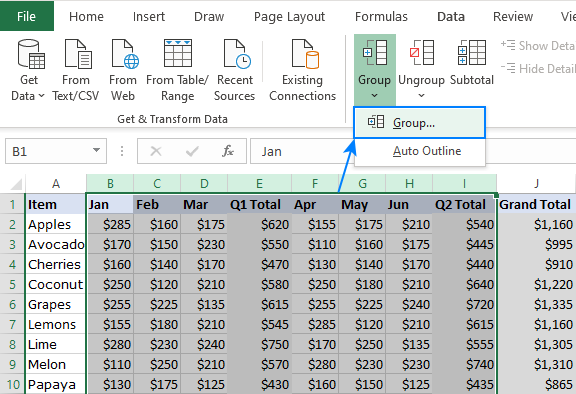
To see how it works in practice, let's group all the intermediate columns in the below dataset. For this, we highlight columns B through I, and click Group:
This creates the level 1 outline like shown below:
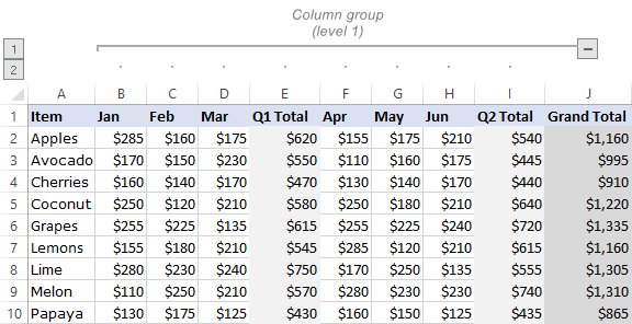
Clicking the minus (-) sign at the top of the group or the outline number 1 in the upper-left corner hides all the columns within the group:

Create nested column groups
Within any group, you can outline multiple groups at inner levels. To create an inner, nested group of columns, this is what you need to do:
- Select the columns to be included in the inner group.
- On the Data tab, in the Outline group, click Group. Or press the Shift + Alt + Right Arrow shortcut.
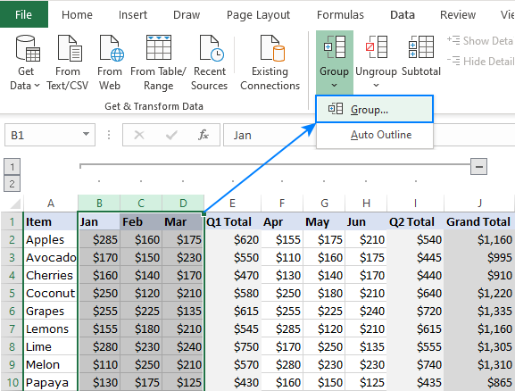
In our dataset, to group the Q1 details, we select columns B through D and click Group:
In the same fashion, you can group Q2 details (columns F through H).
Note. As only adjacent columns can be grouped, you will have to repeat the above steps for each inner group individually.
As the result, we now have 2 levels of grouping:
- Outer group (level 1) - columns B through I
- Two inner groups (level 2) - columns B - D and F - H.
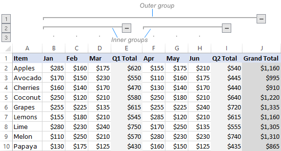
Clicking the minus (-) button above the inner group contracts only that particular group. Clicking the number 2 in the upper-left corner collapses all the groups of this level:

To make the hidden data visible again, expand the column group by clicking the plus (+) button. Or you can expand all the groups at a given level by clicking the outline number.
Tips and notes:
- To quickly hide or show the outline bars and numbers, press the Ctrl + 8 keys together. Pressing the shortcut for the first time hides the outline symbols, pressing it again redisplays the outline.
- If the outline symbols don't show up in your Excel, make sure the Show outline symbols if an outlineis applied check box is selected in your settings: File tab > Options > Advanced category.
How to auto outline columns in Excel
Microsoft Excel can also create an outline of columns automatically. This works with the following caveats:
- There should be no blank columns in your dataset. If there are any, remove them as described in this guide.
- To the right of each group of detail columns, there should be a summary column with formulas.
In our dataset, there are 3 summary columns like show below:

To auto outline columns in Excel, do the following:
- Select the dataset or any single cell within it.
- On the Data tab, click the arrow below Group, and then click Auto Outline.
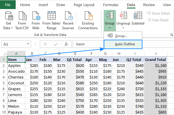
In our case, the Auto Outline feature created two groups for Q1 and Q2 data. If you also want an outer group for columns B - I, you'll have to create it manually as explained in the first part of this tutorial.

If your summary columns are placed to the left of the detail columns, proceed in this way:
- Click a small arrow in the lower-right corner of the Outline group, which is called the dialog box launcher.

- In the Settings dialog box that pops up, clear the Summary columns to right of detail box, and click OK.

After that, use the Auto Outline feature as explained above, and you will get the following result:
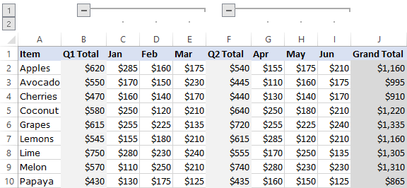
How to hide and show grouped columns
Depending on how many groups you want to cover up or display, use one of the below techniques.
Hide and show a particular column group
- To hide the data within a certain group, click the minus (-) sign for the group.
- To show the data within a certain group, click the plus (+) sign for the group.
Expand or collapse the whole outline to a given level
To hide or show the entire outline to a certain level, click the corresponding outline number.
For example, if your outline has three levels, you can hide all the groups of the second level by clicking the number 2. To expand all the groups, click the number 3.
Hide and show all of the grouped data
- To hide all the groups, click the number 1. This will display the lowest level of detail.
- To display all the data, click the highest outline number. For example, if you have four levels, click the number 4.
Our sample dataset has 3 outline levels:
Level 1 - only shows Items and Grand Total (columns A and J) while hiding all intermediate columns.
Level 2 – in addition to level 1, also displays Q1 and Q2 totals (columns E and I).
Level 3 - shows all the data.

How to copy only visible columns
After hiding some column groups, you may want to copy the displayed data somewhere else. The problem is that highlighting the outlined data in the usual way selects all the data, including the hidden columns.
To select and copy only visible columns, this is what you need to do:
- Use the outline symbols to hide the columns that you don't want copied.
- Select the visible columns using the mouse.
- On the Home tab, in the Editing group, click Find & Select > Go To.
- In the Go To Special dialog box, select Visible cells only, and click OK.
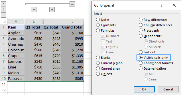
- Now that you have only the visible cells selected, press Ctrl + C to copy them.
- Click the destination cell and press Ctrl + V to paste the copied data.
How to ungroup columns in Excel
Microsoft Excel provides an option to remove all groupings at once or ungroup certain columns only.
How to remove the entire outline
To remove all groupings at a time, go to the Data tab > Outline group, click the arrow under Ungroup, and then click Clear Outline.

Notes:
- Clearing outline only removes the outline symbols; it does not delete any data.
- If some column groups were collapsed while clearing outline, those columns might remain hidden after the outline is removed. To display the data, undie columns manually.
- Once the outline is cleared, it's not possible to get it back with Undo. You will have to recreate the outline from scratch.
How to ungroup specific columns
To remove grouping for certain columns without removing the entire outline, these are the steps to perform:
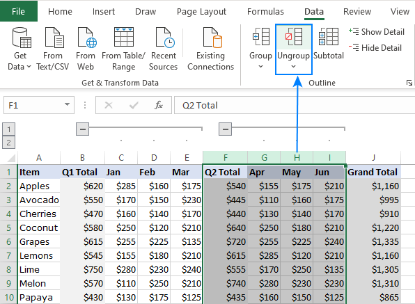
- Select the rows you want to ungroup. For this, you can hold down the Shift key while clicking the plus (+) or minus (-) button for the group.
- On the Data tab, in the Outline group, and click the Ungroup button. Or press the Shift + Alt + Left Arrow keys together, which is the ungrouping shortcut in Excel.
That's how to group and auto outline columns in Excel. I thank you for reading and hope to see you on our blog next week.
 by
by
4 comments
Is there a way to assign a name to "grouped" columns or rows?
Hello Terry!
In Excel, you can’t directly assign a name to grouped columns or rows. However, you can use named ranges to achieve a similar effect. Here’s how you can do it:
1.Select the Range: Highlight the columns or rows you want to group.
2.Name the Range: Go to the “Formulas” tab, click on “Define Name,” and enter a name for your range.
3.Use the Name: You can now refer to this range by the name you assigned in formulas and other Excel features.
In XLXS I have a column with a list of names in alphabetical order. In other columns I have lists of times for events associated with these names. How do I create a column, adjacent to a column of times, that shows the placing i.e. 1st, 2nd, 3rd (or 1,2,3) all the way to the last person. Not all names are in every event. I don't want to sort the sheet as that would change the list of names.
Hello!
If you want to determine the rank of each value, I recommend using the RANK function. Look for the example formulas here: Excel RANK function and other ways to calculate rank.
If this is not what you wanted, please describe the problem in more detail.