In this tutorial, you'll learn 4 easy and quick ways to hide columns in Excel.
Somewhere I read that hiding something is never good as it only makes people more curious about it. Personally, I don't think that hiding things is always bad as it is in our nature. Moreover, this concept is universal. You probably noticed that dogs often hide their food or toys guided by an instinct to guard their possessions. People also have many secrets to hide, such as medical records, credit card numbers, or bad habits.
Read on to see how to hide unwanted columns in an instant with a keyboard shortcut or VBA code, and how to leverage the Group feature to cover-up and expand columns.
Why hide columns in Excel?
The possibility to hide columns in Excel is really helpful. There may be lots of reasons for keeping certain details from showing. For example:
- You wish to view non-adjacent columns side-by-side to compare their data.
- There are a few helper columns in your worksheet with complex formulas that may confuse other users.
- Some columns contain important data that you want to prevent from being seen or edited by your colleagues. See how to lock cells and protect sheets.
Excel shortcut to hide column
The shortcut for hiding columns in Excel is Ctrl + 0.
For the sake of clarity, the last key is zero, not the uppercase letter "O".
- To hide a single column, select any cell within it, then use the shortcut.
- To hide multiple columns, select one or more cells in each column, and then press the key combination.
- To hide non-adjacent columns, click on the header of the first column, press and hold the Ctrl key while clicking on each additional column to select them, and then use the hiding shortcut.
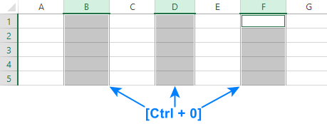
Tip. The shortcut for unhiding columns in Excel is Ctrl + Shift + 0. To make the hidden columns visible, highlight at least one cell in the columns on both sides of the hidden one(s), and use the shortcut. The bad news is that this key combination does not work in some versions of Windows for unknown reasons. In this case, use another method of unhiding columns in Excel.
How to hide columns using a context menu
Don't want to bother remembering the hotkeys? Here's another amazingly simple way to hide columns in Excel:
- Select one or several columns to be hidden.
- Right-click the selection and pick the Hide option from the menu.
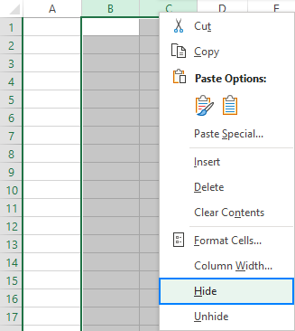
Voila! Now you can easily review your data skipping the extra details.
How to hide a column in Excel using the ribbon
As its name suggests, this option is tucked away deep in the menus, so you need to know where to look for it :)
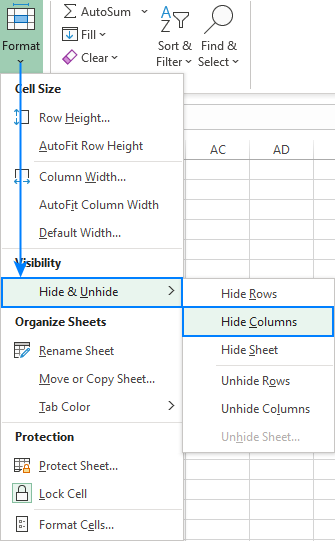
To hide unwanted columns by clicking a ribbon button, the steps are:
- Select the column or any cell within the column(s) you want to hide.
- On the Home tab, in the Cells group, click Format > Hide & Unhide > Hide Columns.
Done! The information that you don't want to view or print is hidden.
How to hide columns in Excel with VBA
Like many other things, hiding columns in Excel can be automated with VBA. In fact, it's a very simple operation, and we'll try to explain the whole concept here.
To do "concealing" programmatically, you can use either the Range or Columns property.
To hide a single column, say column C, the codes are:
Code 1
To specify the column, we use the Range object. To indicate that the entire column should be hidden, the corresponding properties (EntireColumn and Hidden) are added:
Code 2
To hide a column using the Columns property, the code is even simpler:
To hide multiple columns, the codes are essentially the same, except that you specify the first and last columns (A:C in our case).
Code 3
Code 4
To insert the codes in your workbook, please follow these step-by-step instructions: How to insert and run VBA code in Excel. A sample workbook is available for download at the end of this page.
Notes:
- All the codes hide column(s) on the currently open worksheet.
- To hide other columns, change the column letters in the codes.
How to hide unused columns in Excel
To make only the working area of your sheet visible, you can hide all unused (blank) columns to the right of your data. Here's how:
- Select the column to the right of the last column with data.
- Press Ctrl + Shift + Right Arrow to highlight all the unused columns to the end of the sheet.
- Press the Ctrl + 0 key combination to hide the selected columns. Done!
As the result, the workspace is cleaned up and only the relevant information is displayed to the users:

Hide and expand columns using the Group feature
If your worksheet contains a lot of columns, it may be handy organize them in groups to easily show and hide different sections of the sheet. To group columns in Excel, this is what you need to do:
- Select all the columns you want to group, or at least one cell in each column.
- On the Data tab, in the Outline group, click Group (or press the Shift + Alt + Right Arrow keys together).
- If you didn't select entire columns, the Group dialog box will pop up, asking you to select Rows or Columns. Obviously, you choose Columns and click OK.
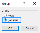
As an example, we are going to group columns B through I that contain item details and monthly sales figures:
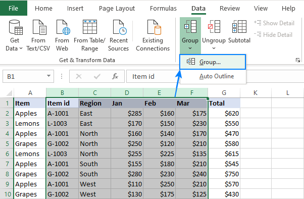
As we've selected the whole columns, clicking the Group button immediately creates the grouping, and the outline symbol appears at the top of the worksheet.
To hide the columns, click on the minus (-) sign above the group.
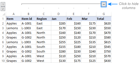
Alternatively, you can collapse and expand groups by using the outline numbers in the upper-left corner. In the screenshot above, clicking on 1 will conceal all the columns between A and G, so that only these two columns are visible.
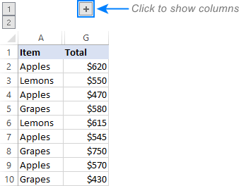
To unhide the columns, click on either the minus (-) sign or the outline number 2:
To remove grouping, do one of the following:
- To ungroup all the columns at any existing levels, go to the Data tab > Outline group, click the arrow under Ungroup, and then click Clear Outline.
- To ungroup specific columns, select those columns, and then click the Ungroup button on the Data tab or press the Shift + Alt + Left Arrow key combination.
Tips and notes:
- Before grouping columns, make sure all the data in your sheet is visible. This will help you avoid incorrect grouping. For more information, please see how to unhide all rows and how to unhide all columns.
- Only adjacent columns can be included in a particular group.
- Within an outer group, you can create any number of inner group levels. For the detailed guidance, please see how to group columns in Excel.
That's how to hide and show columns in Excel. I thank you for reading and hope to see you on our blog next week!
Practice workbook for download
Hide columns in Excel with VBA – code examples (.xlsm file)
 by
by
12 comments
How can I hide column date wise.
E.g.
Column A = Date is 01 JAN
Column B = Date is 02 JAN
Column C = Date is 03 JAN
so on 02 JAN if if open excel 01 JAN column should auto hide and same if i open excel on 03 JAN, 01JAN and 02 JAN should auto hide and continue the same.
Hi! I don't really understand what "open excel 01 JAN column" means. It is possible to automatically hide or show columns using VBA.
How can I create multiple groups of columns that are adjacent, e.g. group a,b,c in one group and d,e,f in another group. The article at https://www.ablebits.com/office-addins-blog/excel-group-rows/#group-rows-outline
Does this for rows.
I am hoping to do this too!
Did ever figure it out?
It works fine for me if the last column in each group is some sort of subtotal column (for example, it SUMS the columns in the group). Without that, the only way I can get it to work is to add a blank column at the end of each group (including the last group, if you are working with a table), then select all the columns in the desired group (including the blank column), then group.
In some ways, this is a bit pointless: when the group is collapsed, all you see is an empty column! And if you subsequently delete the empty column, Excel simply joins the two groups (either side of deleted column) back together. Oh, and if you want to see titles or labels for the groups, put them in the header row at the top of the blank columns. That's what shows when the groups are collapsed.
I get around the annoyance of empty columns by finding something useful to put into them. For example, one of my groups is "Patient data", which contains a bunch of details about each individual. I have populated the "summary" column with data from two of them: "Gender | Age".
It does seem a poor design, based on the core assumption that the primary purpose of Excel is to manage financial (or numerical) data. That may have been valid, even self-obvious, many years ago, but is not the case these days.
Hi
Thank you for the tip. It works great in an unprotected sheet but if i have the sheet protected it doenst allow me to hide the columns. I tried some settings like "format columns" in the selection list when protecting the sheet but this didnt work. Is there a way to protect the sheet and hide/unhide these columns?
Thank you.
Hello, Nico,
Sorry, looks like this is not possible with the standard Excel options.
I have grouped columns on my worksheet but would like to know if I can give the group a name rather than seeing the + and - signs. Is this possible?
Thanks in advance!
Hello, Kay,
Sorr, looks like this is not possible.
hi, same Question as mine, Alternatively what can I do to differentiate the groups
Awesome, Just what I was looking for!
Great instructions!
Thank you so much for your feedback, Danielle,
Happy to know that you found the article helpful.