In case you want to bring focus to top or bottom N values in a dataset, the best way is to highlight them in different colors. This article will teach you how to do this with Excel's presets and set up your own conditional formatting rule based on formula.
Highlighting cells with Excel conditional formatting may sound like a trivial task. But not if you think of how many ways you can actually do it. Do you want to shade the highest or lowest numbers in a range, column, or row? Or maybe you wish to show top 3 values in each row? And it would be really nice if you could control the number of highlighted cells directly on the sheet without having to go to the Conditional Formatting Rules manager every time. This tutorial shows how to do all this and a bit more!
Highlight top or bottom N values in range
In Microsoft Excel, there are a few ways to highlight highest and lowest values with conditional formatting. Below, we provide an overview of 3 different methods, so you can choose the one that works best for you.
Highlight top and bottom values with built-in rule
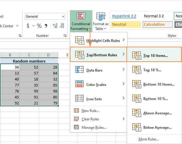
The fastest way to highlight top 3, 5, 10 (or bottom n) values in Excel is to use an inbuilt conditional formatting rule. Here's how:
- Select the range in which you'd like to highlight numbers.
- On the Home tab, in the Styles group, click Conditional Formatting.
- In the drop-down menu, pick Top/Bottom Rules, and then click either Top 10 Items… or Bottom 10 items…

- In the dialog box that opens, specify the number of items to highlight and choose one of the predefined formatting options. To apply formatting that is not in the list, click Custom Format… . The changes you make here are reflected in your dataset immediately. So, if you are happy with the results, click OK.
For this example, we choose to highlight top 3 values with the default Light Red Fill and get this result:

More formatting options to show highest and lowest values
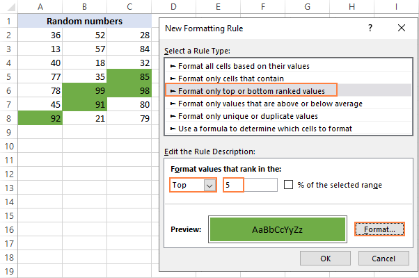
If you want more options than provided in the Top/Bottom presets, you can create a new rule from scratch:
- Select a range with numeric values.
- On the Home tab, click Conditional Formatting > New Rule.
- In the New Formatting Rule dialog box, choose Format only top or bottom ranked values.
- In the drop-down list, select Top or Bottom, and type how many values to highlight in the box next to it.
- Click the Format button and choose any formatting you want for Font, Border and Fill.
- Click OK.
For example, here's how you can highlight top 5 values with a green background color.

Highlight top or bottom values with a formula
The built-in rules described above are handy and easy to apply. However, they have one significant drawback - whenever you want to show a different number of values, you will have to change the number in the Conditional Formatting Rules Manager.
To make the rule more resilient, you can base it on a formula. In our case, we will be using:
LARGE function to shade top numbers:
SMALL function to shade bottom numbers:
To color highest or lowest values by using a formula-based rule, please follow these steps:
- Type the number of values to highlight in a predefined input cell. For this example, we enter the number of top values in F2 and the number of bottom values in F3.
- Select the range of numbers (A2:C8).
- On the Home tab, click Conditional formatting > New Rule.
- In the New Formatting Rule dialog box, select Use a formula to determine which cells to format.
- In the Format values where this formula is true box, enter one of these formulas:
To highlight top n values:=A2>=LARGE($A$2:$C$8, $F$2)To highlight bottom n values:
=A2<=SMALL($A$2:$C$8, $F$3)Where $A$2:$C$8 is the applied range, A2 is the leftmost cell of the range; F2 and F3 are the n values.
Please notice that we lock the source range and input cells with absolute references and use a relative reference for the upper left cell.
- Click the Format button and choose the desired formatting.
- Click OK twice to close both windows.
For more detailed instructions, please see Create a conditional formatting rule with formula.
Done! The top 3 and bottom 3 values are highlighted in different colors.

Later, if you wish to highlight, say, top 5 values, you will just type 5 in F2, and Excel will automatically apply the change.
How this formula works:
The LARGE function returns the n-th largest value in the specified range. In our case, it finds the 3rd largest value in A2:C8, which is 92. The formula compares each number in the selected range with the 3rd highest value. For any cell that is greater than or equal to 92, it returns TRUE, and the conditional formatting rule is applied.
How to shade rows containing top or bottom N values
When analyzing structured data, it may often be helpful to identify entire rows that contain top or bottom n values in the key column. For this, you can configure a formula-based conditional forming rule like explained in the previous example, but the formulas are a bit different.
To show top n rows:
=$B2>=LARGE($B$2:$B$15, $E$2)
To show bottom n rows:
=$B2<=SMALL($B$2:$B$15, $E$3)
Where:
- $B2 is the topmost cell of the numeric column.
- $B$2:$B$15 are the numbers to rank.
- $E$2 is the number of top rows to highlight.
- $E$3 is the number of bottom rows to highlight.
The rules are applied to the whole table except the header row (A2:B15).

Like in the previous example, these rules are flexible. The formulas will recalculate automatically as soon as you change the numbers in the input cells (E2 and E3), and Excel will immediately reflect those changes and highlight a corresponding number of rows.
How to highlight top N values in each row
In case your dataset contains several numeric columns, you may want to show the highest or lowest values in each row. To have it done, you again create an Excel conditional formulating rule using a formula.
For example, to highlight top 3 numbers in each row in the table below, the formula is:
=B2>=LARGE($B2:$G2, 3)
The steps for creating the rule are described in this example, so here we only show the result. The rule is applied to all the numeric cells (B2:G2):

To show bottom 3 rows, the formula would be:
=B2<=SMALL($B2:$G2, 3)
How this formula works:
As you may have noticed, this formula is very similar to the ones used in the previous examples, except the cell and range references. And that little change makes a big difference!
In Excel conditional formatting, references are relative to the upper left cell of the range the rule applies to. So, we can pretend as if we are writing a formula for the leftmost cell, and Excel is "copying" it through all other cells in the selected range.
In this example, the rule is applied to all the numeric cells (B2:G10), but the formula is written for row 2:
=B2>=LARGE($B2:$G2, 3)
The LARGE function finds the 3rd largest value in B2:G2, which is 257. The formula checks if B2 is greater than or equal to 275, and if TRUE, applies the conditional formatting to that cell. Because B2 is a relative reference, Excel then virtually "copies" the formula to C2, D2, etc. As the column coordinates are locked with the $ sign ($B2:$G2), the range does not change when comparing other cells in the same row.
For example, for C2, Excel will be evaluating this formula:
=C2>=LARGE($B2:$G2, 3)
For row 3, the formula automatically changes like shown below because all row coordinates are relative:
=B3>=LARGE($B3:$G3, 3)
And so on.
The following tutorial can help you better understand the inner mechanics: Relative and absolute cell references in conditional formatting.
That's how to highlight top and bottom values in Excel by using conditional formatting. I thank you for reading and look forward to seeing you on our blog next week!
Practice workbook for download
Highlight top or bottom values in Excel (.xlsx file)
 by
by
2 comments
How do you copy conditional formatting down hundreds or thousands of rows? I have a SS with over 8k rows I need to apply formatting to show the highest value in each row.
Hi! Maybe this guide will be helpful: How to copy Excel conditional formatting.