How to use Power Query in Excel – practical examples

Trim and clean

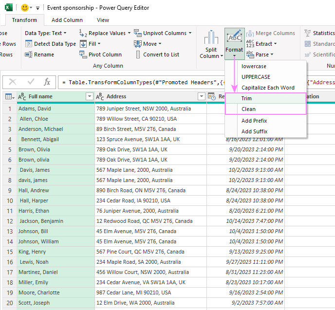
To remove any leading or trailing spaces, or any other unwanted characters, you can use the Trim and Clean functions. Select the columns you want to clean up, go to the Transform tab > Text Column group and click Format > Trim or Clean.

Remove duplicate rows

To eliminate duplicate rows in your data, Power Query offers the Remove Duplicates function. Select the column(s) you want to check for duplicates, then go to the Home tab, and click on Remove Rows > Remove Duplicates.

Remove duplicates case-insensitive

Please keep in mind that this standard "Remove Duplicates" operation will eliminate only the rows that are identical in every way, including the letter case. For a case-insensitive deduplication, you need to modify the M code for the query. Here’s how:

1. Remove case-sensitive duplicates as explained above. Alternatively, you can select and right-click the column that you want to dedupe, and then choose Remove Duplicates from the context menu.
2. In the Formula Bar, add Comparer.OrdinalIgnoreCase as a comparison criterion to the second argument of the Table.Distinct function.

In our case, after doing the standard remove duplicates operation, the Table.Distinct function looked like this:

=Table.Distinct(#"Cleaned Text", {"Full name"})

It successfully removed all the rows with the names in column A that were exactly the same, but it left some entries with variations in letter case, as shown in the screenshot below:

To fix this issue, you can add the Comparer.OrdinalIgnoreCase criterion to the function like this:

=Table.Distinct(#"Cleaned Text", {"Full name", Comparer.OrdinalIgnoreCase})

This will eliminate all the rows containing duplicates in column A, ignoring the letter case.

Users with advanced Excel skills can do this operation in the Advanced Editor by changing the Removed Duplicates line to this format:

Table.Distinct(PreviousStep, {"ColumnName", Comparer.OrdinalIgnoreCase})

Change data type

In case the imported data doesn't look quite right, you can easily convert it into the correct format.

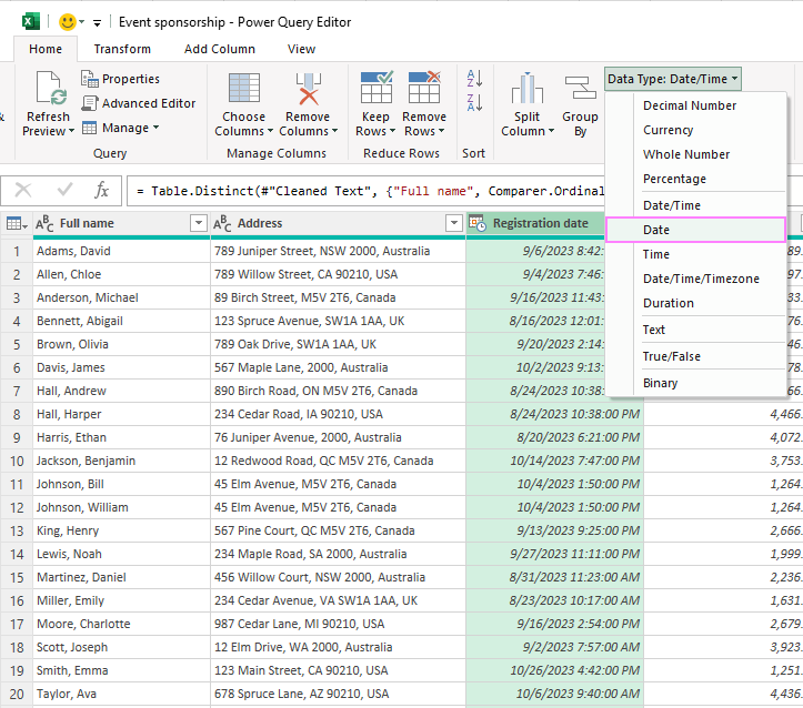
In our sample dataset, the Registration Date column shows both date and time. To display only the date part of the values, you need to change the data type of the column from Date/Time to Date. This can be done in two ways:

• On the Home tab, select Data Type > Date from the ribbon.
• Right-click the column header and choose Change Type > Date.

Custom date format

Power Query applies the default date format from your locale (region settings). To display dates in a custom format, you can use the DateTime.ToText function. Here are the steps to follow:

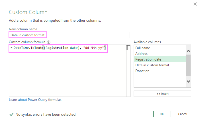
1. On the Add Column tab, in the General group, click Custom Column.
2. In the Custom Column dialog window, type a name for the new column in the corresponding box, e.g. "Date in custom format".
3. In the Custom Column Formula box, enter the DateTime.ToText function with two arguments: the original date column and the custom format code.
   • To add the original date column to the first argument, select it under Available Columns on the right and click Insert, or double click the column name.
   • For the second argument, enter the desired date format such as "dd-MMM-yy" or any other format code.

     The complete formula takes this form:

     =DateTime.ToText([Registration date], "dd-MMM-yy")

4. Click OK, and a new column with the custom date format will be added to your table.

The formula bar will show the complete formula in the M language, which will look something like this:

=Table.AddColumn(#"Previous step", "Date in custom format", each DateTime.ToText([Registration date], "dd-MMM-yy"))

By changing the data type, you can format the values in a more suitable way for your analysis. Similarly, you can change other columns to different data types, such as text, number, or currency, depending on your needs.

Split column

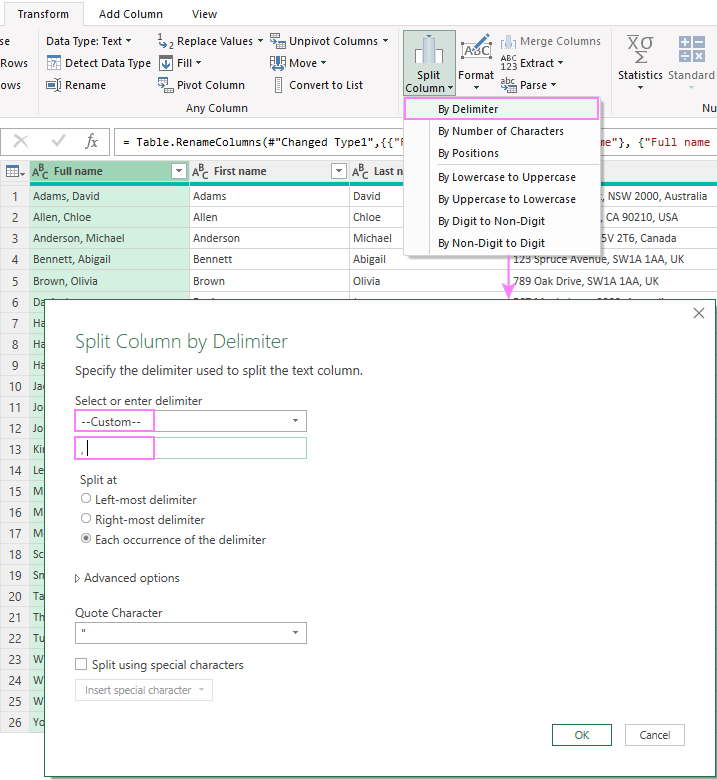
To split a column into two or more columns by a certain delimiter, you can use the Split Column function. For example, to split the "Full Name" column into "First Name" and "Last Name", the steps are:

1. Select the "Full Name" column.
2. Navigate to the Transform tab and, in the Text Column group, click > Split Column > By Delimiter.
3. Pick the delimiter from the dropdown list. If your delimiter is not among the predefined options, choose Custom and enter the desired character(s) in the box below (comma and a space ", " in this example).
4. Decide at which occurrence of the delimiter to separate the column: left-most, right-most or each delimiter. If a cell has only one delimiter, any option will do. But if a cell has more than one delimiter, then you have to choose carefully.
5. When done, click OK.
6. Right-click the header of each new column and choose Rename from the context menu to give them appropriate names (such as "First Name" and "Last Name").

Extract values into a new column

If some column in your dataset contains lengthy multi-part strings, you may want to extract certain information into a new column.

For example, let’s see how to extract the country name from the Address column:

1. Select the column from which you wish to extract values.
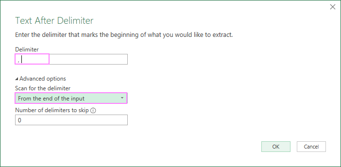
2. Navigate to the Add Column tab, click Extract, and choose an appropriate option. In our case, the country names are separated by a comma, so we choose Text After Delimiter.
3. In the dialog box that pops up, enter the delimiter (a comma and a space ", " in our dataset).
4. Expand the Advanced option section and choose to scan for the delimiter from the end of the input, as the country name comes after the last comma in a cell. If you need to extract a value from the middle of the string, indicate how many delimiters to skip.
5. When done, click OK.

A new column with the extracted values will be added to the end of the table, and you can move it to any position you want by dragging the column header.

Add column from example

When dealing with inconsistent or incomplete data, the standard Split and Extract functions might not work as expected.

Picture a scenario where country names within the Address column are separated by various delimiters like commas, spaces, or vertical bars. In such cases, you can rely on Power Query to extract country names based on an example you provide. This is similar to how Excel's Flash Fill feature works.

Here's how to add a new column using an example from existing columns:

1. Select the column that contains the source data (the Address column in our example).
2. On the Add Column tab, click Column from Examples > From Selection.
3. In the first row of the new column, type the country name that corresponds to the first address. Power Query will try to infer the pattern and fill the rest of the values based on your example. If some cells are blank or filled with incorrect values, provide another example in the second row or any other row until Power Query gets it right.
4. When all the cells are filled with the correct values, press Ctrl + Enter to apply the changes.

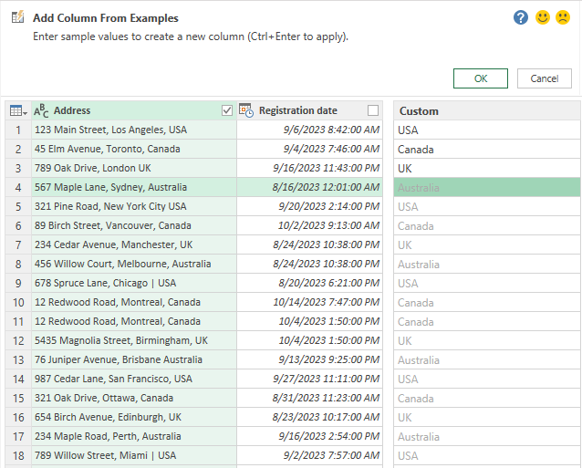
You will now have a new column that extracts the country names from the addresses.

Replace missing values

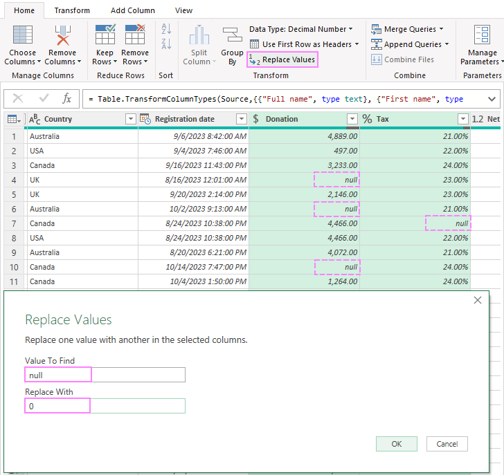
In Power Query, replacing missing values, often represented as null, is a straightforward process:

1. Select the column(s) where you want to handle missing values.
2. On the Home tab, in the Transform group, click Replace Values.
3. In the Replace Values dialog box, fill in two boxes:
   • Value To Find: null
   • Replace With: enter the replacement value corresponding to your data type (e.g., "0" for numeric columns or "N/A" for text columns).
4. Click OK, and Power Query will apply the replacement to all the selected columns.

Add conditional column

To add a new column based on a set of conditions that use existing columns, make use of the Add Conditional Column feature. For example, to add a column that assigns a donor level based on the donation amount, this is what you need to do:

1. Select any column in your dataset.
2. On the Add Column tab, click on Conditional Column.
3. In the dialog box that opens, type Donor Level as the name of the new column. Then, specify the following rules:

   | If Donation | is greater than or equal to | 4000 | then | Platinum |

   | If Donation | is greater than or equal to | 3000 | then | Gold |

   | If Donation | is greater than or equal to | 2000 | then | Silver |

   | Else | Bronze |

4. Click OK to create the new column.

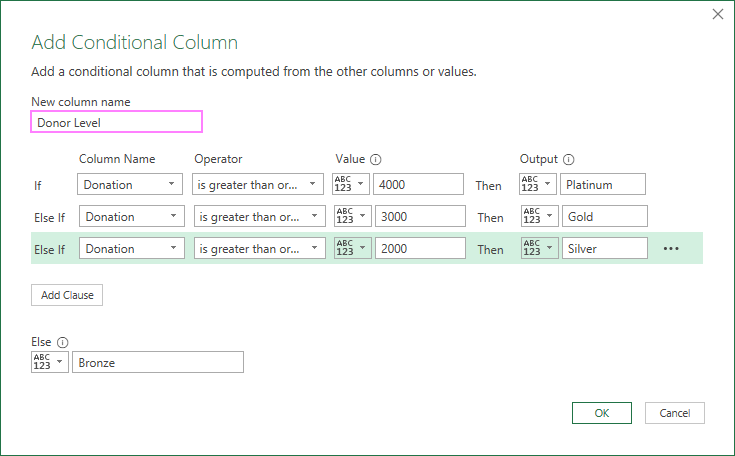
This feature is similar to writing a nested IF statement in Excel, but it’s a lot easier and more convenient to use.

By default, the new conditional column will appear at the end of your dataset, and you can drag it to any position you want.

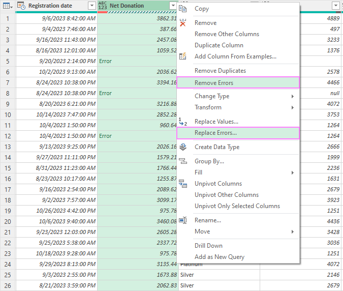
Replace or remove errors

Power Query makes it easy to fix errors in Excel without spending too much time on debugging formulas or VBA code. To eliminate errors in your dataset, follow these simple steps.

1. Select the column where you want to handle errors.
2. Right-click the column header.
3. In the context menu, you'll find two key options for handling errors:
   • Remove Errors will delete all the rows containing errors within the selected column(s), so be careful with this option.
   • Replace Errors will ask you to specify the replacement value. For numeric columns, it has to be a number, e.g. 0. For text columns, you can specify any text value, including a blank cell.

Group and aggregate

To summarize or aggregate data by specific groups, Power Query offers the powerful Group By function.

For example, to calculate the total donation amount by country and donor level, this is what you need to do:

1. On the Home tab, in the Transform group, click on Group By.
2. In the dialog box that opens, choose Advanced Then, do the following:
   • Under Group by, select "Country" and "Donor Level" as the columns to group by.
   • Under New column name, type "Total Donation" as the name of the new column.
   • Under Operation, choose Sum as the aggregation function.
   • Under Column, choose Donation as the column to aggregate.
3. Click OK to apply the changes.

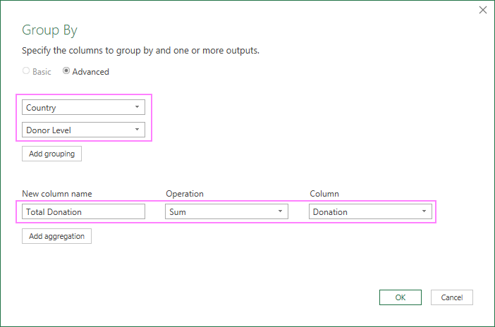
As a result, a new table will be created displaying the grouped and aggregated data. If needed, you can sort the table by one or more columns: right-click the filter arrow next to the column name and choose either to sort ascending or descending.

In this example, we get a summary of total donation amounts based on both country and donor level.

Practice workbook for download

Using Excel Power Query - examples (.xlsx file)