In this article, we will explore the most commonly used formulas in Excel and Google Sheets to check if a value exists in a column, row, or within a range of cells.
Whether you're an experienced user or just starting to learn about your favorite spreadsheet program, knowing how to quickly identify if a specific value is present or absent in a given range can save much time and effort in your data analysis. This can be particularly useful when working with large datasets or when conducting research. In Microsoft Excel and Google Sheets, there are several formulas to perform this task. With our step-by-step guide, you can easily apply them to your spreadsheets, regardless of the structure and size of your dataset.
If value exists in range in Excel
To check if a certain value exists in a range of cells, and if it does then return some text, and if it doesn't then return another text, you can use a combination of the IF and COUNTIF functions.
In this formula, COUNTIF counts the occurrences of a given value in a range. If the count is greater than zero, the IF statement returns "Yes". If the value is not found within the range, the COUNTIF function brings zero, and IF outputs "No".
This generic formula works nicely in all possible scenarios.
Check if value exists in a column
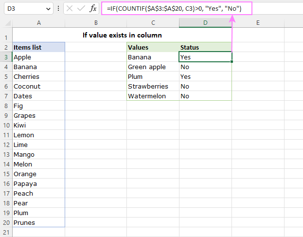
To test if a value in C3 is present in column A (more precisely in the range A3:A20), you can use this formula:
=IF(COUNTIF($A$3:$A$20, C3)>0, "Yes", "No")
Please pay attention that we lock the range reference ($A$3:$A$20) by using the $ sign for the formula to copy correctly in cells D4:D7:
Check if value exists in a row
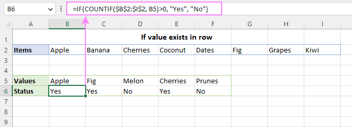
To find out if a value in B5 appears in the row B2:I2, the formula takes this form:
=IF(COUNTIF($B$2:$I$2, B5)>0, "Yes", "No")
Check if value exists in a range
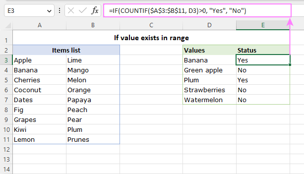
To check if a specific value occurs in a 2D range, supply the corresponding range reference to the first argument of COUNTIF. For example:
=IF(COUNTIF($A$3:$B$11, D3)>0, "Yes", "No")
More formulas to find lookup value in a range
The IF + COUNTIF formula is the easiest but not the only way to find if a certain value appears in a range. Below are a few alternative solutions.
ISNUMBER and MATCH
Another way to check if a value occurs in a list is using MATCH together with the ISNUMBER function. For example:
=IF(ISNUMBER(MATCH(C3, $A$3:$A$20, 0)), "Yes", "No")
The MATCH function returns the position of the lookup value (C3) within the range (A3:A20) as a number; an #N/A error if no match is found. The ISNUMBER function converts a number to TRUE and an error to FALSE. Wrapping the construction into IF gives "Yes" or "No" as the final result.
ISNA and VLOOKUP
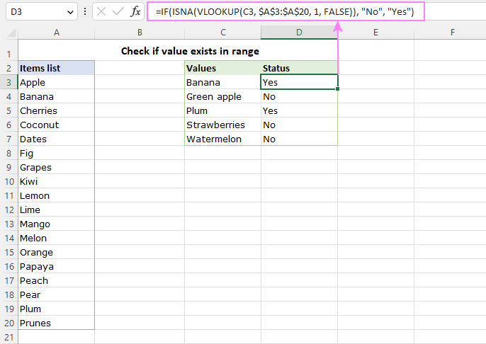
A slightly more complex but still working solution is using the IF, ISNA and VLOOKUP functions in one formula:
=IF(ISNA(VLOOKUP(C3, $A$3:$A$20, 1, FALSE)), "No", "Yes")
Here, the VLOOKUP function searches for the lookup value is the specified array and returns an exact match (FALSE) from the same column (1). If no match is found, an #N/A error is returned. (In Excel 365 and Excel 2021, you can use XLOOKUP instead of VLOOKUP.) The ISNA function checks the result for #N/A errors and returns TRUE if positive, FALSE otherwise. Finally, the IF function returns "No" for TRUE (no match) and "Yes" for FALSE (match).
For more information, please see How to use ISNA with VLOOKUP in Excel.
ISNA and MATCH
This solution is very similar to the previous one except that you utilize MATCH instead of VLOOKUP to check the ranges for matches:
=IF(ISNA(MATCH(C3, $A$3:$A$20, 0)), "No", "Yes")
Tip. If you goal is to find a lookup value in one column and return a matching value from another column, then use the VLOOKUP or XLOOKUP function in its basic form.
If value exists in range in Google Sheets
In Google Sheets, you can check if a value exists in a range using exactly the same formulas that we used in Excel.
For instance, to find whether the value in D3 occurs in the range A3:B11, the formula in E4 is:
=IF(COUNTIF($A$3:$B$11, D3)>0, "Yes", "No")
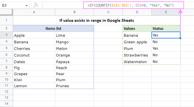
You can find a few more formulas in our sample spreadsheet, which is available at the end of this tutorial.
Check if value exists in range - partial match
To see if any cell in a range contains a given substring, place a wildcard character (asterisk) on both sides of the lookup value so that COUNTIF looks for it anywhere in a cell:
For example, the bellow formula will check if any cell in the range A3:B11 contains the word "apple":
=IF(COUNTIF(A3:B11, "*apple*")>0, "Yes", "No")
If you are referring to a certain cell instead of a hardcoded value, then concatenate asterisks before and after the cell reference like this:
=IF(COUNTIF($A$3:$B$11,"*"&D3&"*")>0, "Yes", "No")

Highlight values that exist in range
A more visual way to identify values that exist in a given range could be highlighting them with Excel Conditional Formatting. The steps are:
- Select the cells with values that you want to find in a range (C3:C7 in our case).
- On the Home tab, in the Styles group, click Conditional Formatting > New Rule.
- In the New Formatting Rule window, select Use a formula to determine which cells to format.
- Enter one of these formulas in the Format values where this formula is true box:
=MATCH(C3, $A$3:$A$20, 0)=COUNTIF($A$3:$A$20, C3)>0Where C3 is the topmost cell with the target values and $A$3:$A$20 is the range to check.
- Click the Format… button and configure the desired formatting.
- Click OK twice to close both dialog windows.
Done! All the values that exist in the range (exact match) are highlighted:

To highlight partially matching values, modify the formula like shown below - concatenate an asterisk on both sides of the lookup value reference:
=MATCH("*"&C3&"*", $A$3:$A$20, 0)
=COUNTIF($A$3:$A$20, "*"&C3&"*")>0

Tip. The same formula can be used with Google Sheets Conditional Formatting to highlight exact or partial matches in a range in Google spreadsheets.
Now you are equipped with the knowledge and skills to check if a value exists in a column, row or range with confidence and ease. Thank you for reading!
Practice workbooks
Check if value exists in range in Excel (.xlsx file)
Find if value exists in range in Google Sheets (online sheet)
 by
by
16 comments
Hi ? I have 5 columns, in column A i have repeatative dates, in column B i have vehicles number(100s of vehicles coming every day), in column C i have quantities of material which vehicles are carrying, in column D i have dates again(on which the specific vehicles get late), in column E i have vehicles number which are late.
Now i want a formula to check the date and vehicle number from column D and Column E and match it with column A and column B and if both date and vehicle numbers get match then in a new column revert the quantity from column C and also i want to highlight rows from A1 to E1
Hello Rahul!
If I understand your question correctly, then you can use the IF AND formula with two conditions. The formula might look like this:
=IF(AND(A1=D1,B1=E1),C1,"")
To highlight cells by this condition, select the range you want (for example, A1:E100) and create a conditional formatting with a formula:
=AND($A1=$D1,$B1=$E1)
The following tutorial should help: Relative and absolute cell references in Excel conditional formatting.
Hi,
Can you remind me the formula to use when I need information from two columns to be true?
For example, Column A in my spreadsheet has the status of something (i.e., Completed)
Column B has the data it was completed (i.e., 12 April 2024)
I want to write a formula that will count for me:
Status from Column A = Completed
AND
Status from Column B = (date in the month of April 2024)
So essentially a date range from April 1-30 and status completed.
I can get these independent of one another but having a hard time doing one formula with both.
I am working in Google Sheets.
Thank you so much!!
Hi Elizabeth,
You'll find formula examples for your case in this article: Google Spreadsheet COUNTIF with multiple criteria
In my Google Sheet, I have a column for the number of students and a column for the scores the students received on a test. Students can receive a 4, 3, 2, or 1 on the test and I am using the =COUNTIFS(C5:C33,"=4") function to find out how many "4s" I have in the column. This data is placed in a row called "Received a 4." If, for instance, 18 of the students received a 4 on the test, then the "Received a 4" row will show the figure 18.
The problem I run into and am trying to fix is in a different row, when I want to find the % of my students (that took the test) that received a 4 on the test. Currently, I am using this formula -- =Round(C35/$A$33, 2), but it takes into account all 29 of my students. Sometimes, on a test, not all 29 students will be present. What I would like the Round cell to compute is, if a student was present, its total will be used in the computation of the %. If a student is not present and a score is not entered into the system for that student, then he/she will not be counted in the total that gives me the percentage.
Can anyone help me with a formula that will take into account only cells that have information in them, instead of using all of the students when I try to compute the percentage?
Thank you for all of your help.
Trigg
Hello Trigg,
I replied to your comment under this article for Google Sheets regarding your task with students' grades. Have you tried that solution? Or has your task gotten more complicated? Please let me know if you still need help with it.
Hello!
I use google sheets for work and am not well versed in formulas, I am hoping someone will be able to help me.
I am wondering if there is a way to mark a checkbox as true in one sheet if it is checked off as true in a master list.
For example, if John's treatment plan for the month of October is completed, I would like to check it off only once from the master list, and it will automatically check off the Treatment Plan column for John every time he is seen in the month.
I hope that is easy to understand, I would appreciate any help. Thank you.
Hello Garcia,
If I understand your task correctly, you need to use the IF function to check whether the checkbox in the master list is TRUE or FALSE, like this:
=IF(MasterSheet!A2=TRUE,TRUE,FALSE)
And then insert a checkbox to a cell with this IF formula as well.
I have a long list of dates in column A and a long list of decreasing loan balance values in Column C. I’m looking for a formula that will provide the date in column A that corresponds to the column C value when it falls between 0 and 1180, there will only be one row that column C meets that value range.
Hi! If I understand your task correctly, the following tutorial should help: Excel INDEX MATCH with multiple criteria - formula examples. The formula below will do the trick for you:
=INDEX(A1:A20,MATCH(1,(C1:C20>0)*(C1:C20<1180),0))
I want to highlight complete selected row, If value match with other sheet single column.
Hi! If I understand your task correctly, the following tutorial should help: Apply conditional formatting to entire rows in Google Sheets.
I haven't seen these types of creative solutions before. They don't quite fix my problem but I would be most appreciated if I could be pointed in the right direction. I need the row of a value to use for an indirect value formula. I need to find "First Quarter" in another sheet using importrange and the row that it is in. I am unsure how to do this as all my efforts have failed thus far. Thank you kindly in advance.
John Mak
Hello John,
Since you mentioned IMPORTRANGE, I assume you work in Google Sheets. If so, I believe the QUERY function will help you with your task.
Hi
I am having troubles with an equation. Maybe someone is smart enough to help me.
I want excel to look for a value in a cell that is in a range of numbers (for example 0.10 to 0.99) whenit picks up the number within the range it must display a specific word as well.
The catch is that I will have to display these words according to the value found within the range.
Cell C3 is a value that the user will punch in manualy. I want Cell D3 to tell me if C3 is a value within 0.01 and 0.20 then display F40. There will be multiple of these equations in one cell and I simply can't get them to work.
Example =if(C3>0.01,C3<=0.20,"F40")
Hi! If I understand your task correctly, try the following formula:
=IF(AND(C3>0.01,C3<=0.20),"F40")
You can also find useful information in this article: Nested IF in Excel – formula with multiple conditions.