In this tutorial, you will learn how to quickly insert current time in Excel using a shortcut, formula, or VBA macro. Also, we'll look at how to convert timestamp to date and get hours, minutes or seconds from a timestamp.
There are a number of ways to insert time into Excel worksheets. Which one to use depends on whether you want a static timestamp or a dynamic value that updates automatically to reflect the current date and time.
How to insert time in Excel using shortcut
To insert the current time into an Excel cell as a static timestamp, use one of the following keyboard shortcuts:
- To insert current time, press Ctrl + Shift + ;
- To enter current date and time, press Ctrl + ; which inserts a date, then press the Space key, and then hit Ctrl + Shift + ; to insert the current time.
The result is a static value that won't change when a workbook is recalculated.
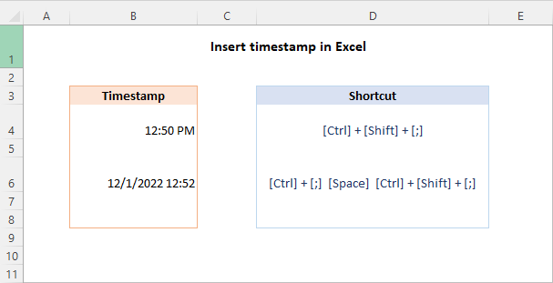
Tip. The timestamp is inserted in the default date/time format. To have the date and time displayed differently, change the Number format applied to the cell. For more information, please see Excel date format and Excel time format.
Insert current time as static value with VBA
Another way to insert the current date and time in Excel as a static value without auto-updating is by using VBA. Here's how:
- Insert the following code in the Visual Basic Editor. The detailed instructions are here: How to add VBA code in Excel.
Sub NowFunction() Application.ActiveCell.Value = Now() End Sub
- Create a button from a shape or any other graphic object and link the macro to the button as explained in this example: How to make a macro button in Excel.
- Select the cell where you want to insert the date and/or time as a static value.
- Click the macro button.
- Apply the desired time format to the cell. Done!
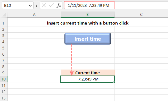
On the below image, the cell is formatted to display only time, but the formula bar shows the entire date time value, which was returned by the macro and is now stored in the cell.
Tip. You can also make Excel NOW function static by creating a custom function.
Insert current date and time using NOW function
If you aim to insert the current date and time as a dynamic value that refreshes automatically, then use the Excel NOW function.
The formula is as simple as it can possibly be, no arguments are required:
=NOW()
Like the timestamp shortcuts, the NOW function inserts the current date and time in the default format defined in your Region settings. You can easily change this by applying a custom date and time format.
Here are a few examples of how the Excel NOW function results can be formatted:
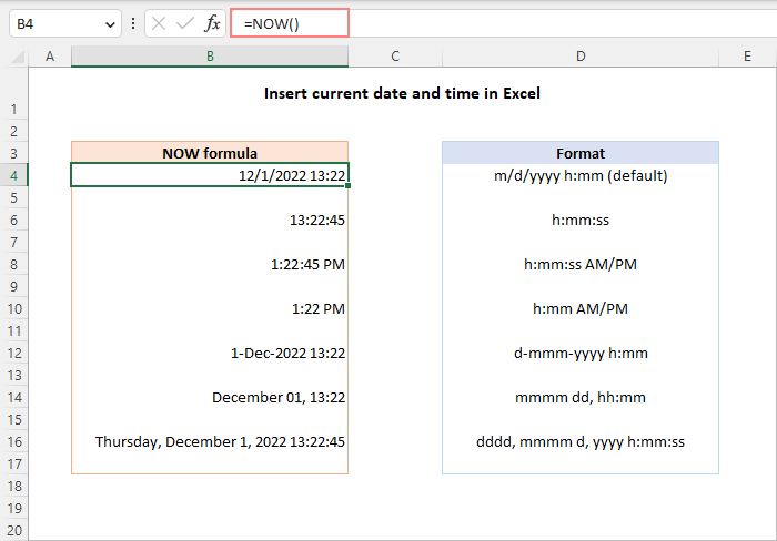
When using the NOW function in Excel, there are a few things to keep in mind:
- The time is retrieved from your computer's system clock.
- NOW is a volatile function that recalculates every time the worksheet is re-opened or recalculated.
- To force a NOW formula to update, press either Shift + F9 to recalculate the active worksheet or F9 to recalculate all open workbooks.
For more details, please see How to use NOW function in Excel.
Insert current time as dynamic value
If you wish to insert only the current time without a date, you have the following choices:
- Format NOW formula to only show time.
Use a regular NOW formula, and then apply the time format you want to the result:
=NOW()Please remember, this will only change the display representation. The actual value stored in a cell will still be a decimal number consisting of an integer representing the date and a fractional part representing the time.
- Return only the time value.
Make use of the INT function to round the decimal number returned by NOW() down to the nearest integer. And then, subtract the integer part representing today's date so that only the fractional part representing the current time is output.
=NOW() - INT(NOW())Another option is to subtract the integer part representing the date (returned by TODAY) from the date time value (returned by NOW):
=NOW() - TODAY()By default, both formulas return a decimal number representing the time internally in Excel. To get a correct result, apply the Time format to the cell.
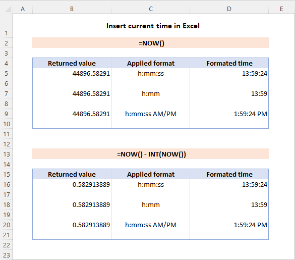
The following screenshot demonstrates both formulas in action. Pay attention that although the formatted time values look the same (column D), the actual values stored in cells (column B) are different - the results returned by the second formula (B16:B20) contain only the fractional part.
Insert current hour in Excel
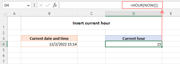
To insert the current hour as a number between 0 (12:00 AM) and 23 (11:00 PM), use the HOUR and NOW functions together:
=HOUR(NOW())
Yep, it's that simple :)
How to convert Excel timestamp to date
Assume you have a column of timestamps in your worksheet from which you wish to remove the time value and keep only the date. This can be done in a few different ways.
Format timestamp to only show date
The easiest way to convert a timestamp to a date is to format it in such a way that only a date is visible in a cell. Here's how:
- Select the cell(s) with the time stamps.
- Press Ctrl + 1 to open the Format Cells dialog box.
- On the Number tab, select Date or Custom in the Category list, and then either choose one of the predefined date formats from the Type list or enter your own format code in the box.
- When done, click OK.
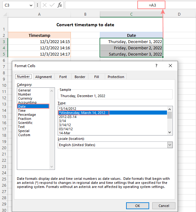
If you'd rather have a date in a separate cell, enter a formula like =A3 (where A3 is the original timestamp) in any empty cell in the same row, and set the Date format for that cell.
For example, here's how you can change a timestamp to the default long date format:
Remove time from timestamp
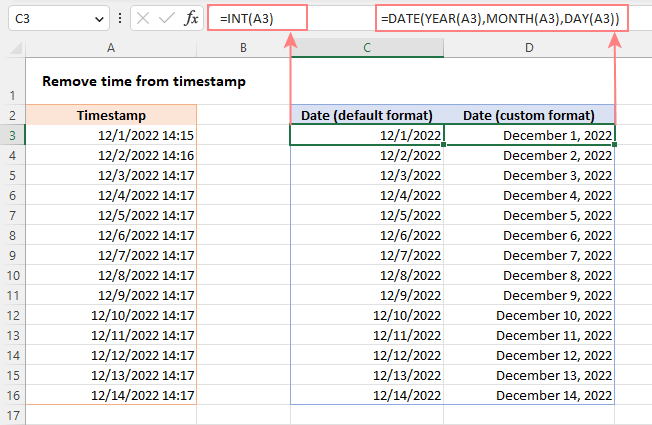
In Excel's internal system, a date time value is stored as a decimal number where time is represented by a fractional part. An easy way to remove that part is using the INT function that rounds a decimal down to the integer:
=INT(A3)
Or you can extract the date with the help of the DATE function:
=DATE(YEAR(A3), MONTH(A3), DAY(A3))
Whichever formula you choose, set the Date format for the formula cells and you'll get the result you are looking for:
Note. All the methods described above assume a timestamp is a date time value and not a text string. If your timestamp is a text value, then you need to convert text to date first. Or you can split a text string into different columns, or extract a substring representing the date.
How to get hours, minutes and seconds from timestamp
To extract a specific time unit from a time stamp, you can use the following functions:
HOUR(serial_number) - returns an hour of a time value, as an integer from 0 (12:00 am) to 23 (11:00 pm).
MINUTE(serial_number) - gets the minutes of a time value, as an integer from 0 to 59.
SECOND(serial_number) - returns the seconds of a time value, as an integer from 0 to 59.
In all three functions, serial_number can be supplied as a reference to the cell containing the time, text string enclosed in double quotes (for example, "6:00 AM"), decimal number (e.g. 0.25 representing 6:00 AM), or the result of another function.
In the image below, the following formulas are used.
To return hours from the timestamp in A2:
=HOUR(A2)
To get minutes from the timestamp in A2:
=MINUTE(A2)
To extract seconds from the timestamp in A2:
=SECOND(A2)

How to insert specific time in Excel
When you type a time value in a cell, in most cases Microsoft Excel recognizes it as such and automatically applies the Time format. If Excel does not understand what you are entering, the TIME function can help. The syntax is intuitive and straightforward:
The hour, minute and second arguments can be provided as numbers from 0 to 32767. The supplied numbers are processed in this way:
- If hour is greater than 23, it is divided by 24 and the remainder is taken as the hour value.
- If minute is greater than 59, it is converted to hours and minutes.
- If second is greater than 59, it is converted to hours, minutes, and seconds.
For example:
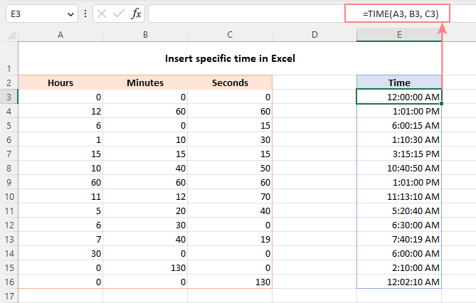
- TIME(30, 0, 0) equates to TIME(6, 0, 0), which is 6:00 AM.
- TIME(0, 130, 0) is converted to TIME(2, 10, 0), which is 2:10:00 AM.
- TIME(0, 0, 130) is converted to TIME(0, 2, 10), which is 12:02:10 AM.
The Excel TIME function is particularly useful when it comes to combining individual units into a single time value.
Assuming you have hours in A3, minutes in B3 and seconds in C3, the following formula will put them together:
=TIME(A3, B3, C3)
That's how to insert the current date and time in Excel with shortcuts and formulas. I thank you for reading and hope to see you on our blog next week!
Practice workbook for download
Insert time in Excel - examples (.xlsx file)
 by
by
5 comments
Sub NowFunction()
Application.ActiveCell.value = Now()
End Sub
What would be the function just for the time and not the date?
Hi! To use VBA to insert the current time, use the Time function.
Sub NowFunction()
Application.ActiveCell.Value = Time
End Sub
I need to analyse data in my spreadsheet.
We had a summer play scheme.
I have the days and AM/PM SESSIONS in the columns across the top.
In the rows I have the children's names, ages and the sessions which they attended (ticked if they attended).
I need to know: Numbers of children attending the AM sessions up to and including age 6yrs.
Please can you help with a formula for this as I then have to do 7+ years
so the layout is like this:
Monday Tuesday Wednesday
Name Age AM PM AM PM AM PM
Dan 6 (tick) (tick)
Hope that makes sense.
Can you please help.
Thanks
Lucy
Hi! If I understand the question correctly, you can use the SUMPRODUCT function to find the sum based on the conditions in the rows and columns of the table.
=SUMPRODUCT(C3:J10*(B3:B10<N1)*(C2:J2=P1))
P1 = "AM"
N1 = 7
I hope my advice will help you solve your task.
sorry - the above format is not very clear - the top line is the day then under it is the AM/PM for each day!