The tutorial shows six different ways to insert a tick in Excel and explains how to format and count cells containing checkmarks.
There are two kinds of checkmarks in Excel - interactive checkbox and tick symbol.
A tick box, also known as checkbox or checkmark box, is a special control that allows you to select or deselect an option, i.e. check or uncheck a tick box, by clicking on it with the mouse. If you are looking for this kind of functionality, please see How to insert checkbox in Excel.
A tick symbol, also referred to as check symbol or check mark, is a special symbol (✓) that can be inserted in a cell (alone or in combination with any other characters) to express the concept "yes", for example "yes, this answer is correct" or "yes, this option applies to me". Sometimes, the cross mark (x) is also used for this purpose, but more often it indicates incorrectness or failure.
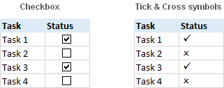
There are a handful of different ways to insert a tick symbol in Excel, and further on in this tutorial you will find the detailed description of each method. All of the techniques are quick, easy, and work for all versions of Microsoft Excel 2016, Excel 2013, Excel 2010, Excel 2007 and lower.
How to put a tick in Excel using the Symbol command
The most common way to insert a tick symbol in Excel is this:
- Select a cell where you want to insert a checkmark.
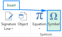
- Go to the Insert tab > Symbols group, and click Symbol.
- In the Symbol dialog box, on the Symbols tab, click the drop-down arrow next to the Font box, and select Wingdings.
- A couple of checkmark and cross symbols can be found at the bottom of the list. Select the symbol of your choosing, and click Insert.
- Finally, click Close to close the Symbol window.
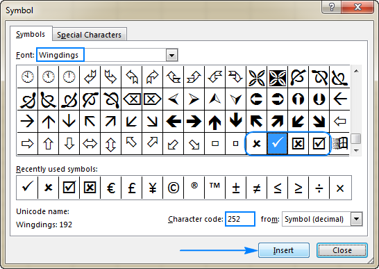
Tip. As soon as you've selected a certain symbol in the Symbol dialog window, Excel will display its code in the Character code box at the bottom. For example, the character code of the tick symbol (✓) is 252, as shown in the screenshot above. Knowing this code, you can easily write a formula to insert a check symbol in Excel or count tick marks in a selected range.
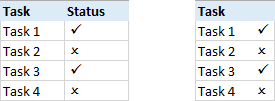
Using the Symbol command, you can insert a checkmark in an empty cell or add a tick as part of the cell contents, as shown in the following image:
How to insert tick in Excel using the CHAR function
Perhaps it's not a conventional way to add a tick or cross symbol in Excel, but if you love working with formulas, it may become your favorite one. Obviously, this method can only be used for inserting a tick in an empty cell.
Knowing the following symbol codes:
| Symbol | Symbol Code |
| Tick symbol |
252 |
| Tick in a box |
254 |
| Cross symbol |
251 |
| Cross in a box |
253 |
The formula to put a checkmark in Excel is as simple as this:
=CHAR(252) or =CHAR(254)
To add a cross symbol, use either of the following formulas:
=CHAR(251) or =CHAR(253)
Note. For the tick and cross symbols to be displayed correctly, the Wingdings font should be applied to the formula cells.
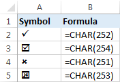
One you've inserted a formula in one cell, you can swiftly copy a tick to other cells like you usually copy formulas in Excel.
Tip. To get rid of the formulas, use the Paste Special feature to replace them with values: select the formula cell(s), press Ctrl+C to copy it, right-click the selected cell(s), and then click Paste Special > Values.
Insert tick in Excel by typing the character code
Another quick way to insert a check symbol in Excel is typing its character code directly in a cell while holding the Alt key. The detailed steps follow below:
- Select the cell where you want to put a tick.
- On the Home tab, in the Font group, change font to Wingdings.
- Press and hold ALT while typing one of the following character codes on the numeric keypad.
| Symbol | Character Code |
| Tick symbol |
Alt+0252 |
| Tick in a box |
Alt+0254 |
| Cross symbol |
Alt+0251 |
| Cross in a box |
Alt+0253 |
As you may have noticed, the character codes are the same as the codes we used in the CHAR formulas but for leading zeros.
Note. For the character codes to work, make sure NUM LOCK is on, and use the numerical keypad rather than the numbers at the top of the keyboard.
Add tick symbol in Excel using keyboard shortcuts
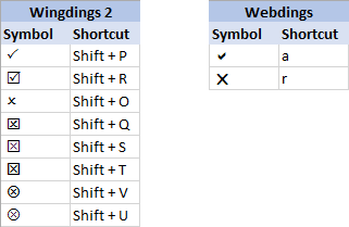
If you do not particularly like the appearance of the four check symbols we have added so far, check out the following table for more variations:
| Wingdings 2 | Webdings | ||
| Shortcut | Tick symbol | Shortcut | Tick symbol |
| Shift + P | a | ||
| Shift + R | r | ||
| Shift + O | |||
| Shift + Q | |||
| Shift + S | |||
| Shift + T | |||
| Shift + V | |||
| Shift + U | |||
To get any of the above tick marks in your Excel, apply either Wingdings 2 or Webdings font to the cell(s) where you want to insert a tick, and press the corresponding keyboard shortcut.
The following screenshot shows the resulting checkmarks in Excel:
How to make a checkmark in Excel with AutoCorrect
If you need to insert tick marks in your sheets on a daily basis, none of the above methods may seem fast enough. Luckily, Excel's AutoCorrect feature can automate the work for you. To set it up, perform the following steps:
- Insert the desired check symbol in a cell using any of the techniques described above.
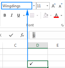
- Select the symbol in the formula bar and press Ctrl+C to copy it.

Don't be discouraged by the appearance of the symbol in the formula bar, even if it looks differently from what you see in the screenshot above, it just means that you inserted a tick symbol using another character code.
Tip. Look at the Font box and make a good note of the font theme (Wingdings in this example), as you will need it later when "auto-inserting" a tick in other cells.
- Click File > Options > Proofing > AutoCorrect Options…
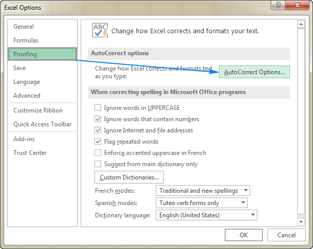
- The AutoCorrect dialog window will open, and you do the following:
- In the Replace box, type a word or phrase that you want to associate with the check symbol, e.g. "tickmark".
- In the With box, press Ctrl+V to paste the symbol that you copied in the formula bar.
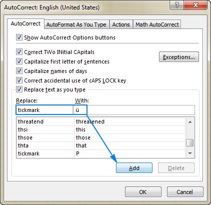
- Click Add, and then click OK to close the AutoCorrect dialog window.
And now, whenever you want to put a tick in your Excel sheet, do the following:
- Type the word that you linked with the checkmark ("tickmark" in this example), and press Enter.
- The symbol ü (or some other symbol that you copied from the formula bar) will appear in a cell. To turn it into an Excel tick symbol, apply the appropriate font to the cell (Wingdings in our case).
The beauty of this method is that you have to configure the AutoCorrect option only once, and from now on Excel will be adding a tick for you automatically every time you type the associated word in a cell.
Insert tick symbol as an image
If you are going to print out your Excel file and want to add some exquisite check symbol to it, you can copy an image of that check symbol from an external source and paste it into the sheet.
For example, you can highlight one of the tick marks or cross marks below, press Crl + C to copy it, then open your worksheet, select the place where you want to put a tick, and press Ctrl+V to paste it. Alternatively, right-click a tick mark, and then click "Save image as…" to save it on your computer.
Tick marks Cross marks
![]()
![]()
![]()
![]()
![]()
![]()
Tick symbol in Excel - tips & tricks
Now that you know how to insert a tick in Excel, you may want to apply some formatting to it, or count cells containing the checkmarks. All that can be easily done as well.
How to format checkmark in Excel
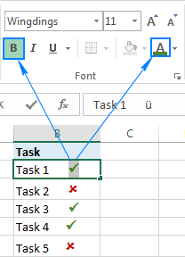
Once a tick symbol is inserted in a cell, it behaves like any other text character, meaning that you can select a cell (or highlight only the check symbol if it's part of the cell contents), and format it to your liking. For example, you can make it bold and green like in the screenshot below:
Conditionally format cells based on the tick symbol
If your cells do not contain any data other than a tick mark, you can create a conditional formatting rule that will apply the desired format to those cell automatically. A big advantage of this approach is that you will not have to re-format the cells manually when you delete a tick symbol.
To create a conditional formatting rule, perform the following steps:
- Select the cells that you want to format (B2:B10 in this example).
- Go to the Home tab > Styles group, and click Conditional Formatting > New Rule…
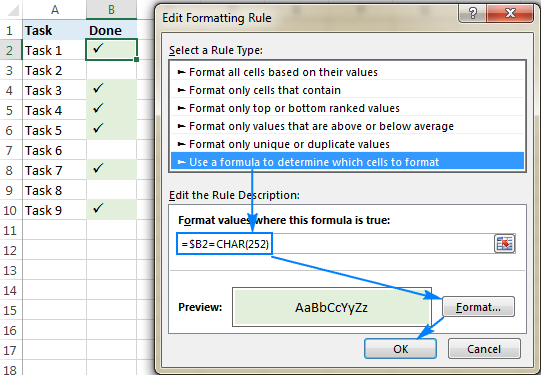
- In the New Formatting Rule dialog box, select Use a formula to determine which cells to format.
- In the Format values where this formula is true box, enter the CHAR formula:
=$B2=CHAR(252)Where B2 is the topmost cells that can potentially contain a tick, and 252 is the character code of the tick symbol inserted in your sheet.
- Click on the Format button, choose the desired formatting style, and click OK.
The result will look something similar to this:
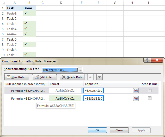
In addition, you can conditionally format a column based on a tick mark in another cell in the same row. For example, we can select the task items range (A2:A10) and create one more rule with the strikethrough format using the same formula:
=$B2=CHAR(252)
As the result, the completed tasks will be "crossed off", like shown in the screenshot below:
Note. This formatting technique works only for the tick symbols with a known character code (added via the Symbol command, CHAR function, or Character code).
How to count tick marks in Excel
Experienced Excel users must have got the formula up and running already based on the information in the previous sections. Anyway, here's a hint - use the CHAR function to detect the cells containing a check symbol, and the COUNTIF function to count those cells:
=COUNTIF(B2:B10,CHAR(252))
Where B2:B10 is the range where you want to count check marks, and 252 is the check symbol's character code.
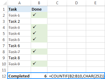
Notes:
- As is the case with conditional formatting, the above formula can only handle tick symbols with a specific character code, and works for cells that do not contain any data other than a check symbol.
- If you use Excel tick boxes (checkboxes) rather than tick symbols, you can count the selected (checked) ones by linking check boxes to cells, and then counting the number of TRUE values in the linked cells. The detailed steps with formula examples can be found here: How to make a checklist with data summary.
This is how you can insert, format and count tick symbols in Excel. No rocket science, huh? :) If you also want to learn how to make a tick box in Excel, be sure to check out the following resources. I thank you for reading and hope to see you on our blog next week.
 by
by
46 comments
Hi,
I previoused that about correct ticks formula is really helpful also I am wondering about additional for incorrect cross and percentage for total with formula.
'=COUNTIF(B1:B20,CHAR(252)) - tick
'=COUNTIF(B1:B20,CHAR(253)) - cross
?? - percentage total %
thank you
Hi! Sorry, it's not quite clear what you are trying to achieve.
Thank you, great advice!!!!
Great article. Many thanks to publishing this. I have a related but different question.
In addition to the techniques mentioned here, you can also use the Developer tab in Excel to add a checkbox to any cell. By default the checkbox has a tick mark, which is not particularly visible. I want to change that default tick mark to an X for all checkboxes in the spreadsheet but cannot find any way to do that. Any suggestions?
Ok, I know this thread is old, but I guess people here might have a clue. Have you seen how checkboxes work in Google Sheets? I'm desperately trying to find a way to emulate that feature/behavior. It's really easy to check and return a TRUE value. But I can't fin a satisfying solution in the MS Office 365 environment. Any ideas?
Hi, If I already have checkboxes, how do I place a green checkmark or a red "x" in these boxes, depending for example, if a test passed or failed, I want to have a green check in the box when pass and a red x when fail. Could someone please help. Thank you!!
Hello!
Here is the article that may be helpful to you: Excel conditional formatting Icon Sets, Data Bars and Color Scales.
I hope it’ll be helpful.
Thank U so much
Thanks for this! Makes it easier to put symbols not existing on our keyboards.
THANKS
Hi
i have an existing Excel spreadsheet and i need to add a tick and yes once i have entered the data CHAMPNESS, John 1040235 3/08/2020
DA SILVA, Roberto 1083557 27/07/2020 28/07/2020 30 ü YES
i have tried all your examples but i cant work out how to do it?? Have tried multiple times and i need your advice how to get the tick and word yes at the end cells. Hope you can help me? Thanks Sue
I was trying but unable to find tick mark
how to insert tick mark inside existing box in excel, please can any one explain me in detail.
Thanks,
Vidya
Please transfer for arbaic
What symbol works with window ten.
°F gives °F
Hi Svetlana,
Character codes above 127 seems to be specific to each machine (Windows installation). Is there a more universal methods of inserting special characters from within a formula? Unicode perhaps? For instance, in your examples above for CHAR(252) I am getting not "check mark" but a letter with diacritical mark.
Thanks / Alex M
Hi Alex,
For CHAR(252) to work, the Wingdings font should be set for the formula cell. Sorry, I don't know any other way to insert tick marks with formulas.
It really helps. :) Good job.
Hi - Is there a to autocorrect the text to tick without changing the font. i.e. Cutting the 2 steps process (1. enter the text 2. change the font of the text entered) to one step.
Hi Ablebits team
I have set up simulate the behavior of the form control checkbox when using Excel Online? Given that form controls are not supported by the online version of Excel.
i.e. I would like the user to check the box with a mouse click rather than using wingdings or other characters. The user may viewing in a Browser or on the iOS Excel App.
Many thanks
Richard
Puted good effort. Great work. It's my 1st time I commented on any website, keep it up.
Hi I have recently taken over a spread sheet at work. When I write a 0 a picture of a cross appears and when I type any other nunber a picture of a tick appears. There is no formulary in the cells. I have no idea how this was done. Can anyone help? Thanks
How do I link tick box cells (Which I have set up and the cell with text in also turns green when i tick the tick box) But what I'm trying to do is link that to a cell at the end with "C" & "D" in thumbs up or down. So when all the boxes are ticked I get the thumbs up!.
Any help is much appreciated.
So I understand how to make the check in the boxes however what if it is a box I am wanting someone to fill out. Can someone simply click the box for it to check? Or would they have to go to insert?
Hi Ash,
In case you are using the Check Box control, then of course check boxes can be ticked off and cleared by simply clicking the box.