Today we will continue exploring MIN function and find out some more ways of finding the smallest number based on one or multiple conditions in Excel. I'll show you the combination of MIN and IF and then tell you about the brand-new MINIFS function to prove that this one is definitely worth your attention.
I've already narrated about the MIN function and its capabilities. But if you have been using Excel for some time, I believe you know that you can combine formulas with one another in many ways to solve as many different tasks as you may only think of. In this article, I'd like to continue making our acquaintance with MIN, show you some more ways of using it and offer an elegant alternative.
Shall we begin?
MIN with several conditions
A while back I showed you the usage of MIN and IF functions so that you could find the smallest number on the basis of some criterion. But what if one condition is not enough? What if you need to conduct a more complex search and locate the lowest value based on a few requirements? What should you do then?
When you know how to discover a minimum with 1 limitation using MIN and IF, you may wonder about the ways to detect it by two or even more parameters. How can you do that? The solution would be as obvious as you think – using MIN and 2 or more IF functions.
So, in case you need to find the lowest quantity of apples sold in a particular region, here is your solution:
{=MIN(IF(A2:A15=F2,IF(C2:C15=F3,D2:D15)))}
Alternatively, you may avoid multiple IFs by using the multiplication symbol (*). Since you apply an array formula, the AND operator is replaced with an asterisk. You may check this page to refresh your knowledge about logical operators in array functions.
Thus, the alternative way to get the smallest number of apples sold in the south would be the following:
{=MIN(IF((A2:A15=F2)*(C2:C15=F3),D2:D15))}
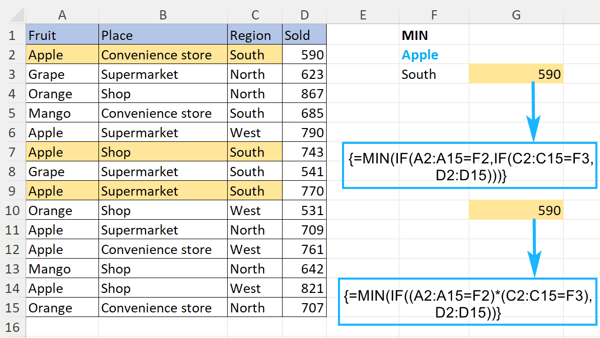
Note! Remember that the combination of MIN and IF is an array formula which should be entered by Ctrl + Shift + Enter.
MINIFS or how to easily find the smallest number based on one or several conditions
MINIFS returns the minimum value by one or multiple guidelines you specify. As you can see from its name, this is a combination of MIN and IF.
Note! This function is available only in Microsoft Excel 2019 and in the newest versions of Office 365.
Explore the syntax of MINIFS
This formula goes through your data range and returns you the smallest number according to the parameters you set. Its syntax is as below:
- Min_range (required) - the range to find the minimum in
- Range1 (required) - the set of data to check for the first requirement
- Criteria1 (required) - the condition to check Range1 for
- [range2], [criteria2], … (optional) - additional data range(s) and their corresponding requirements. You are free to add up to 126 criteria and ranges in one formula.
Remember us looking for the littlest number using MIN and IF and hitting Ctrl + Shift + Enter to turn it into the array formula? Well, Office 365 users have another solution available. Spoiler alert – it's easier :)
Let's get back to our examples and check how easy the solution may be.
Use MINIFS to get a minimum by one criterion
The charm of MINIFS is in its simplicity. Look, you show it the range with numbers, a set of cells to check for the condition and the condition itself. It's easier done than said actually :)
Here is the new formula to solve our previous case:
=MINIFS(B2:B15,A2:A15,D2)
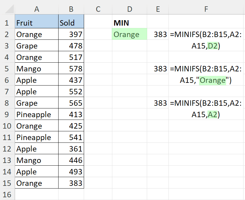
The logic is as simple as ABC:
A - First goes the range to check for the minimum.
B - Then the cells to look the parameter in and the parameter itself.
C - Repeat the last part as many times as there are criteria in your formula.
Find a minimum on the basis of multiple conditions with MINIFS
I showed you the way to locate the lowest number determined by 1 requirement using MINIFS. It was pretty easy, right? And I believe by the time you finish reading this sentence, you'll realize that you already know how to locate the smallest number by several criteria :)
Here is an update for this task:
=MINIFS(D2:D15, A2:A15, F2, C2:C15, F3)
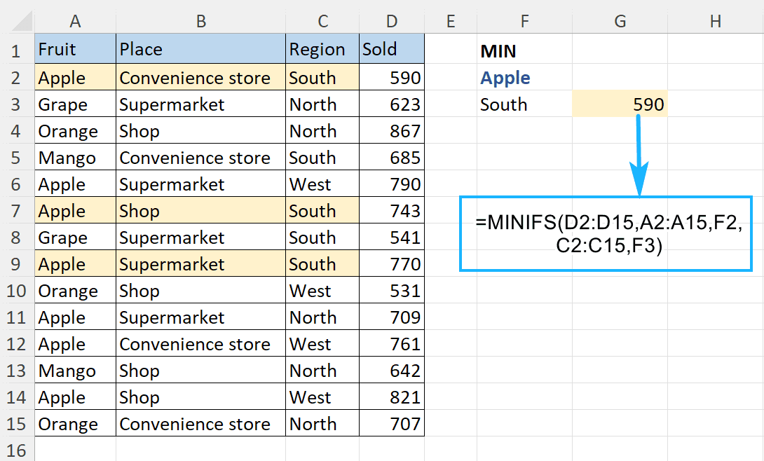
Note! The size of min_range and all the criteria_range must be the same so that the formula works correctly. Otherwise, you'll get the #VALUE! error instead of the correct result.
How to find the smallest number without zeroes using MINIFS
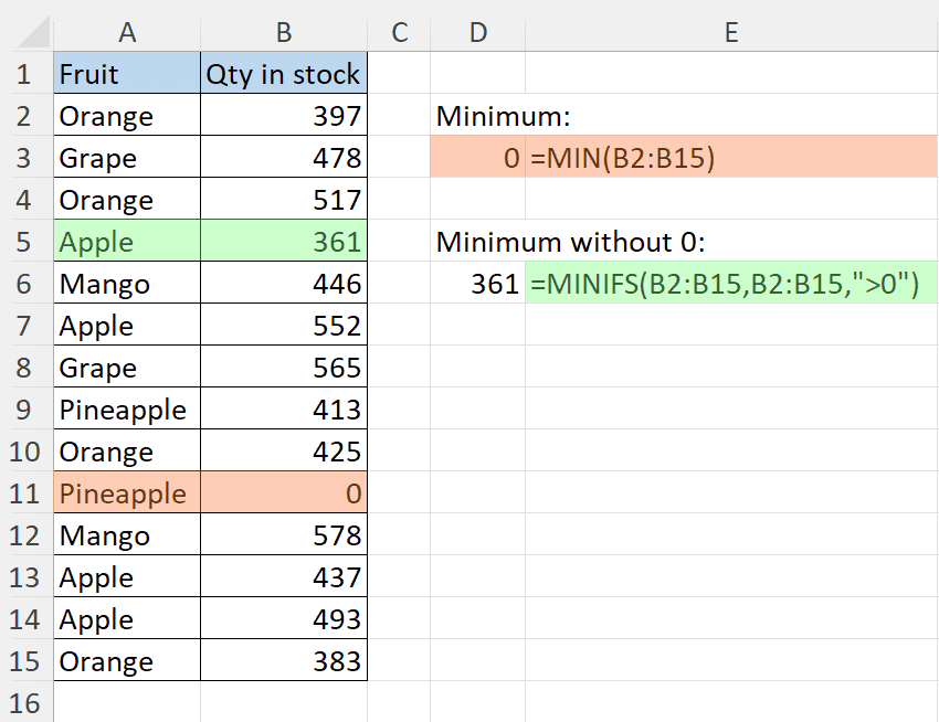
The parameters you specify in MINIFS may be not only some words and values, but also expressions with logical operators (>,<,<>,=). I'm saying that you can locate the smallest figure that is more than zero using just one formula:
=MINIFS(B2:B15, B2:B15, ">0")
Using MINIFS to locate the smallest value by a partial match
When locating the bottom number, it may turn out that your search is not entirely accurate. There may be some extra words, symbols or accidental spaces after the keyword in your data range that may prevent you from getting the expected result.
Luckily, wildcards may be used in MINIFS and be your little savers in this situation. So, if you know for sure that there are multiple different entrances of, let's say, apples in your table and you need to find the smallest figure of all, just put an asterisk right after the search word so that the formula looks like this:
=MINIFS(C2:C15,A2:A15,"Apple*")
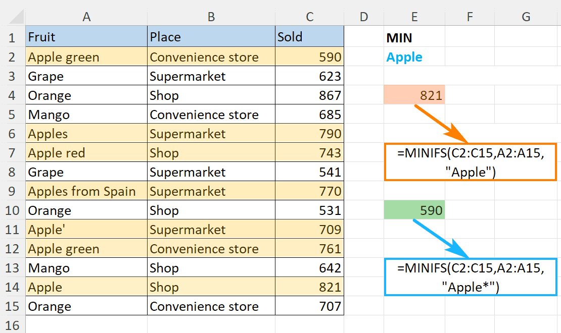
In this case, it will check all the occurrences of apple followed by any words and symbols and return you the smallest number from the Sold column. This trick may become a real time and nerve saver when it comes to partial matches.
They say "Old is gold". But as far as you can see something new (like MINIFS) may be even better. It is simple, effective and there is no need to keep in mind the Ctrl + Shift + Enter combination all the time. Using MINIFS you can easily find the smallest value based on one, two, three, etc. conditions.
But if you prefer the "old gold", the MIN and IF pair will do the trick for you. It will take a few more button clicks, but it works (isn't it the point?)
If you are looking to find Nth lowest value with criteria, use the SMALL IF formula.
I hope you enjoyed your reading today. In case you have any questions or other examples in mind, please leave your thoughts in the comments section.
 by
by
6 comments
I have read your article How to use MINIFS function in Microsoft Excel.
I have also tried all the eksamles in the article.
But on of the aksamples give me a different answer than shown.
The eksample is "Find a minimum on the basis of multiple conditions with MINIFS" about in the midddel.
I'm suppose to get the answer 590 but I get 0.
I'm using Win11 and office 2019.
I'm from Denmark, so I have used danish Excel and the proper danish functions and so on.
BR
Torben
Hi! The MINIFS function in Danish Excel is MIN.HVIS.SET. The syntax is similar to the English version, requiring the range to find the minimum, followed by criteria ranges and conditions.
Hello,
I'm working with MINIFS function and need your help with one piece. Column F is the date range, column A is the location range, column C is the employee range and column B is the appointment type range.
=MINIFS(F3:F2359,A3:A2359,"Brighton",C3:C2359,"Phillip",B3:B2359,"Any 15")
this works great as long as all the criteria is met, but if one of the criteria isn't met the answer is a default date of 1/0/1900 and I would like the answer to be N/A.
Thank you.
Hello Brenda!
The result you get is the number 0 in date format. If you want the formula to return the text “N/A” instead of 0, try using the IF function.
For example:
=IF(MINIFS(F3:F2359,A3:A2359,"Brighton",C3:C2359,"Phillip",B3:B2359,"Any 15")=0, "N/A", MINIFS(F3:F2359,A3:A2359,"Brighton",C3:C2359,"Phillip",B3:B2359,"Any 15"))
I want to use the MIN IF function to find the fastest total time for different types of boats in different age classes for a race where the total times are greater than 24 hours. However, I keep getting a 0:00:00 result every time. - Example data would be Column A: Cell A1 - "Boat_Type" (Cell A2:A5 - "K1", Cell A6:A10 - "K2"; Column B: Cell B1 - "Class", Cell B2:B10 - "O Open", "O Open", "O Open", "O V40", "O V50", "O Open", "O V40", "X Open", "X Open", "W Open", and Column C: Cell C1 - "Total_Time", Cells C2:C10- "28:32:45", "28:42:21", "29:45:53", "29:01:23", "30:17:34", "27:45:52", "28:32:40", "28:18:43", "29:52:44", "31:01:23". So I want to find the fastest Total time for a K1, O Open, or a K2, W Open, etc. How do I do it? I want to be able expand this concept to find records (the fastest times) from over 50 years of data (one spreadsheet for each year), and each year having hundreds of entries covering many boat types, and classes.
Hello!
I hope you have studied the recommendations in the tutorial above. It contains answers to your question. To find the fastest time for Boat_Type use the MINIFS function:
=MINIFS(C2:C10,A2:A10,"K1")
For two criteria, the MINIFS formula is -
=MINIFS(C2:C10,A2:A10,"K1",B2:B10,"O Open")
I hope I answered your question.