We continue learning basic operations with columns in Google Sheets. Learn how to move and hide columns to operate the datasets more efficiently. Also, you will find out how to lock a column (or more) and merge them in order to create a powerful table.
How to move columns in Google Sheets
Sometimes when you work with tables you may need to relocate one or a couple of columns. For example, move information that is more important to the beginning of the table or place columns with similar records beside one another.
- Before you start, select a column as you did previously. Then choose Edit > Move column left or Move column right from the Google Sheets menu:
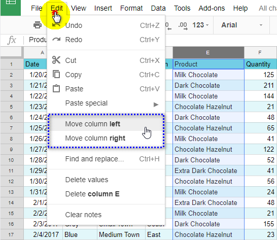
Repeat the same steps to move the column further if necessary.
- To move records a few columns left or right at once, select a column and hover the cursor over the column heading until the former turns into a hand icon. Then click it and drag to the desired position. An outline of the column will help you track the position of the column-to-be:
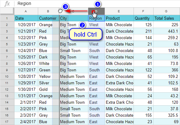
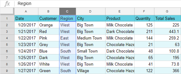
As you can see, we moved column D left and it became column C:
How to merge columns in Google Sheets
Not only does Google let you move columns, but also merge them. This can help you create beautiful column headers or enclose large pieces of information.
Though merging cells is a more common and required feature, I think it's important to know how to merge columns in Google Sheets as well.
Note. I advise you to merge columns before entering any data into a table. When you merge columns, only the values in the leftmost column will remain.
However, if the data is already there, you can use our Merge Values for Google Sheets. It joins values from multiple columns (rows and cells as well) into one.
Select columns you want to merge, A and B, for instance. Then select Format > Merge cells:
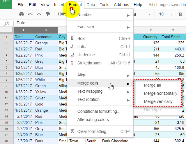
This option offers the following choices:
- Merge all - combines all cells in the range.
All values except the one in the top leftmost cell are deleted (A1 with the word "Date" in our example). - Merge horizontally - the number of rows in the range won't change, the columns will be merged and filled with the values from the leftmost column of the range (column A in our example).
- Merge vertically - merges cells within each column.
Only the top value of each column is preserved (in our example it is "Date" in A1 and "Customer" in B2).
To cancel all the merging, click Format > Merge cells > Unmerge.
Note. The Unmerge option won't restore the data lost during merging.
How to hide columns in Google Sheets
If you work with loads of data, chances are you have helpful columns needed for calculations but not necessarily for displaying. It would be much better to hide such columns, don't you agree? They won't distract from the main information yet provide numbers for formulas.
To hide a column, select it beforehand. Click the button with a triangle to the right of the column letter and choose Hide column:
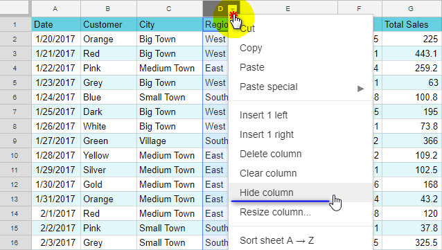
Hidden columns will be marked with small triangles. To unhide columns in Google Sheets, one click on any of the triangles will do the trick:

Freeze and unfreeze columns in Google Sheets
If you work with a large table, you may want to lock or "freeze" its parts so they're always seen on your screen when you scroll down or right. That part of the table can contain headers or other important information that helps read and navigate the table.
The most common column to lock is the first one. But if a few columns include important information, you may need to lock them all. You can do that in one of the following ways:
- Select any cell from the column you want to freeze, go to View > Freeze, and choose how many columns you'd like to lock:
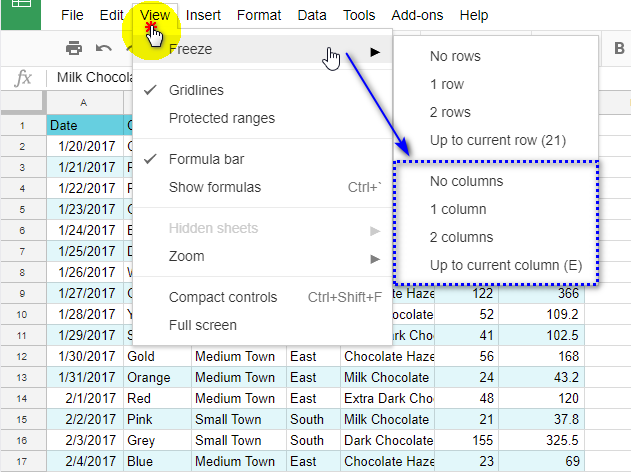
As you can see, you can freeze many columns in Google Sheets. Just make sure your screen is wide enough to show them all at once :)
- Hover the cursor over the right border of the grey box that joins columns and rows. When the cursor turns into a hand icon, click it and drag the borderline that appears one or more columns to the right:
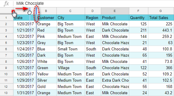
The columns to the left of the border will become locked.
Tip. To cancel all the actions and return the table to its initial state, go to View > Freeze > No columns.
This is it, now you know how to move, hide and unhide, merge and freeze columns in Google Sheets. Next time I'll introduce you to some fancier features. Hope you'll be here to meet them!
 by
by
6 comments
I have 1.25 sheets for my resume. I just want 1 sheet. How can I move .25 sheet into the first sheet so my resume is only one sheet
Hello Karen,
I'm sorry, I'm afraid I don't quite understand your task. Could you please describe it in detail? Do you need to combine data from the sheets into one sheet?
Hi, EXAMPLE: I have the name of a person in column C and I have a dollar amount in column D. I need to transfer this data alone with its correspondent name to column A ( for the dollar amount from column D ) and into column B ( its correspondent person of column C ). can you please help?
Hi Carlos,
Perhaps, these ways to concatenate data will help you out. If this is not exactly what you need, please provide examples of your source cells (C and D) and of what you need to appear in other cells (A and B).
Sir,
Required a formula if a cell contains a word in that word 4th Letter P = individual and if it C = corporate
Hello, Govind,
If your cell with a word is A2, then use the following:
=IF((MID(A2;4;1))="P";"individual";IF((MID(A2;4;1))="C";"corporate";""))
You can learn more about the IF function in Google Sheets from this article of ours:
https://www.ablebits.com/office-addins-blog/if-function-google-sheets/#combination-other-functions
Hope this helps!